7 Modeling as a Process

7.1 Comparing Models³

So many models, so little time. Understanding how to interpret a multiple linear regression model is only half of the modeling process. In most real-life situations, there are many variables which can be used to predict or describe the response variable at hand. But how to choose which combination or subset of variables is best?

Here, we’ll walk through many of the big ideas surrounding the modeling building process. In the next chapter we will consider the technical ideas behind statistical inference for modeling building. But even when using formal inference, the ideas here should always inform the larger process and analysis conclusions.

Leo Breiman was among the giants in machine learning who helped to bridge ideas in statistics and computer science. Trained as a statistician, he spent his career at the University of California, Berkeley where he developed Classification and Regression Trees (CART), bagging, and Random Forests.

Among his important insights was an idea that there are two cultures which can motivate (linear) modeling:

Think of the data as being generated by a black box in which a vector of input variables x (independent variables) go in one side, and on the other side the response variables y come out. Inside the black box, nature functions to associate the predictor variables with the response variables.

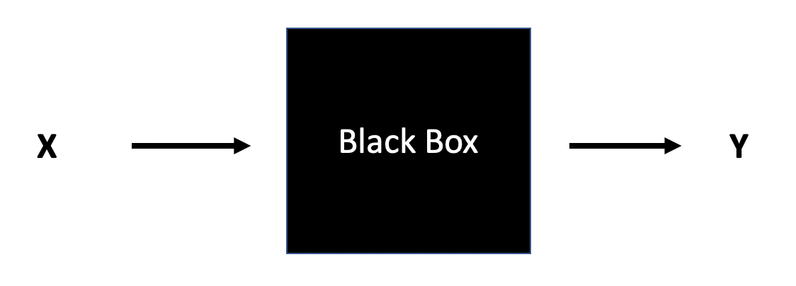
Data Modeling: The analysis in this culture starts with assuming a stochastic data model for the inside of the black box…The values of the parameters are estimated from the data and the model then used for information and/or prediction

Algorithmic Modeling: The analysis in this culture considers the inside of the box complex and unknown. [The] approach is to find a function f(x) — an algorithm that operates on x to predict the responses y.

Here in Chapter 7, the focus will be on algorithmic modeling and developing models which are optimally predictive of the response variable at hand.

Spoiler:

In Chapter 6, the model building uses hypothesis testing and p-values.
In Chapter 7, the model building uses outside information and independent assessment.

There isn’t a right way to model. In fact, good data analysis is hard. You are building a tool box. Make sure to notice that not every tool is the same, and you have more than just one hammer to use. Sometimes the tools can work together to form even better models.

Worth a comment

Notice that the R code has gotten more interesting now. How fun!! The R code will help the process! The R package tidymodels includes tools to facilitate, in particular, feature engineering and cross validation.

Bias-variance trade-off

Excellent resource

for explaining the bias-variance trade-off: http://scott.fortmann-roe.com/docs/BiasVariance.html

Variance refers to the amount by which \(\hat{f}\) would change if we estimated it using a different training set. Generally, the closer the model fits the data, the more variable it will be (it’ll be different for each data set!). A model with many many explanatory variables will often fit the data too closely.
Bias refers to the error that is introduced by approximating the “truth” by a model which is too simple. For example, we often use linear models to describe complex relationships, but it is unlikely that any real life situation actually has a true linear model. However, if the true relationship is close to linear, then the linear model will have a low bias.

Generally, the simpler the model, the lower the variance. The more complicated the model, the lower the bias. In this class, cross validation will be used to assess model fit using metrics like accuracy and Receiver Operating Characteristic (ROC) curves.

\[\begin{align} \mbox{prediction error } = \mbox{ irreducible error } + \mbox{ bias } + \mbox{ variance} \end{align}\]

irreducible error The irreducible error is the natural variability that comes with observations. No matter how good the model is, we will never be able to predict perfectly.
bias The bias of the model represents the difference between the true model and a model which is too simple. That is, the more complicated the model (e.g., the more variables), the closer the points are to the prediction. As the model gets more complicated (e.g., as variables are added), the bias goes down.
variance The variance represents the variability of the model from sample to sample. That is, a simple model (very few variables) would not change a lot from sample to sample. The variance decreases as the model becomes more simple (e.g., variables are removed).

Note the bias-variance trade-off. We want our prediction error to be small, so we choose a model that is medium with respect to both bias and variance. We cannot control the irreducible error.

Test and training error as a function of model complexity. Note that the error goes down monotonically only for the training data. Be careful not to overfit!! [@ESL]

Figure 2.1: Test and training error as a function of model complexity. Note that the error goes down monotonically only for the training data. Be careful not to overfit!! (Hastie, Tibshirani, and Friedman 2001)

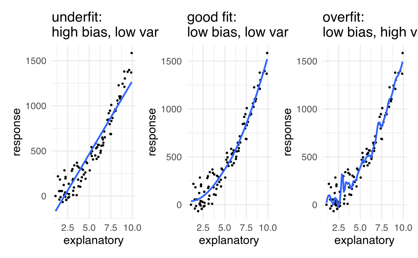
In the linear regression case, the following plots describe the bias-variance tradeoff. In our setting, the models change due to the number of variables included in the model (which is difficult to draw because those models exist in dozens of dimensions).

7.2 Modeling Squirrel Activity

For the example used to consider feature engineering and cross validation, the data come from Project FeederWatch#TidyTuesday dataset on Project FeederWatch, a citizen science project for bird science, by way of TidyTuesday. Many of the ideas below are due to screencasts by Julia Silge.

Can the characteristics of the bird feeder site like the surrounding yard and habitat predict whether a bird feeder site will be used by squirrels?

Instead of jumping into the predictions immediately, let’s look at the data itself. What wrangling can we do to the data in order to take advantage of all the information in the variables? We’d also like to make the model accurate and easy to communicate.

site_data <- read_csv('https://raw.githubusercontent.com/rfordatascience/tidytuesday/master/data/2023/2023-01-10/PFW_count_site_data_public_2021.csv') %>%
  mutate(squirrels = as.factor(ifelse(squirrels, "squirrels", "no squirrels")))

glimpse(site_data)
#> Rows: 254,355
#> Columns: 62
#> $ loc_id                       <chr> "L100016", "L100016", "L100016", "L100016…
#> $ proj_period_id               <chr> "PFW_2002", "PFW_2003", "PFW_2004", "PFW_…
#> $ yard_type_pavement           <dbl> 0, 0, 0, 0, 0, 0, 0, 0, 0, 0, 0, 0, 0, 0,…
#> $ yard_type_garden             <dbl> 0, 0, 0, 0, 0, 0, 0, 0, 0, 0, 0, 0, 0, 0,…
#> $ yard_type_landsca            <dbl> 1, 1, 1, 1, 1, 1, 0, 0, 0, 0, 1, 1, 1, 1,…
#> $ yard_type_woods              <dbl> 0, 0, 0, 0, 0, 0, 1, 1, 1, 1, 1, 1, 1, 1,…
#> $ yard_type_desert             <dbl> 0, 0, 0, 0, 0, 0, 0, 0, 0, 0, 0, 0, 0, 0,…
#> $ hab_dcid_woods               <dbl> 1, 1, 1, 1, 1, 1, 1, 1, 1, 1, NA, NA, NA,…
#> $ hab_evgr_woods               <dbl> NA, NA, NA, NA, 0, 0, NA, NA, NA, NA, NA,…
#> $ hab_mixed_woods              <dbl> 1, 1, 1, 1, 1, 1, NA, NA, NA, NA, 1, 1, 1…
#> $ hab_orchard                  <dbl> NA, NA, NA, NA, 0, 0, NA, NA, NA, NA, NA,…
#> $ hab_park                     <dbl> NA, NA, NA, NA, 0, 0, NA, NA, NA, NA, 1, …
#> $ hab_water_fresh              <dbl> 1, 1, 1, 1, 1, 1, 1, 1, 1, 1, 1, 1, 1, 1,…
#> $ hab_water_salt               <dbl> NA, NA, NA, NA, 0, 0, NA, NA, NA, NA, 1, …
#> $ hab_residential              <dbl> 1, 1, 1, 1, 1, 1, NA, NA, NA, NA, 1, 1, 1…
#> $ hab_industrial               <dbl> NA, NA, NA, NA, 0, 0, NA, NA, NA, NA, 1, …
#> $ hab_agricultural             <dbl> 1, 1, 1, 1, 1, 1, NA, NA, NA, NA, 1, 1, 1…
#> $ hab_desert_scrub             <dbl> NA, NA, NA, NA, 0, 0, NA, NA, NA, NA, NA,…
#> $ hab_young_woods              <dbl> NA, NA, NA, NA, 0, 0, NA, NA, NA, NA, NA,…
#> $ hab_swamp                    <dbl> NA, NA, NA, NA, 0, 0, NA, NA, NA, NA, NA,…
#> $ hab_marsh                    <dbl> 1, 1, 1, 1, 1, 1, NA, NA, NA, NA, 1, 1, 1…
#> $ evgr_trees_atleast           <dbl> 11, 11, 11, 11, 11, 11, 0, 0, 0, 4, 1, 1,…
#> $ evgr_shrbs_atleast           <dbl> 4, 4, 4, 4, 1, 1, 1, 1, 1, 1, 4, 4, 4, 4,…
#> $ dcid_trees_atleast           <dbl> 11, 11, 11, 11, 1, 1, 11, 11, 11, 11, 4, …
#> $ dcid_shrbs_atleast           <dbl> 4, 4, 4, 4, 4, 4, 11, 11, 11, 11, 4, 4, 4…
#> $ fru_trees_atleast            <dbl> 4, 4, 4, 4, 1, 1, 1, 1, 1, 1, 1, 1, 1, 1,…
#> $ cacti_atleast                <dbl> 0, 0, 0, 0, 0, 0, 0, 0, 0, 0, 0, 0, 0, 0,…
#> $ brsh_piles_atleast           <dbl> 0, 0, 0, 0, 0, 0, 1, 1, 1, 1, 1, 1, 1, 1,…
#> $ water_srcs_atleast           <dbl> 1, 1, 1, 1, 1, 1, 0, 0, 0, 0, 0, 0, 0, 0,…
#> $ bird_baths_atleast           <dbl> 0, 0, 0, 0, 0, 0, 1, 1, 1, 1, 0, 0, 0, 1,…
#> $ nearby_feeders               <dbl> 0, 1, 1, 1, 0, 0, 1, 0, 1, 1, 1, 1, 1, 1,…
#> $ squirrels                    <fct> no squirrels, no squirrels, no squirrels,…
#> $ cats                         <dbl> 0, 1, 1, 1, 1, 1, 1, 0, 0, 0, 1, 1, 1, 1,…
#> $ dogs                         <dbl> 0, 0, 0, 0, 0, 0, 1, 0, 0, 0, 1, 1, 1, 1,…
#> $ humans                       <dbl> 0, 0, 0, 0, 0, 1, 1, 1, 0, 1, 1, 1, 1, 1,…
#> $ housing_density              <dbl> 2, 2, 2, 2, 2, 2, 1, 1, 1, 1, 2, 2, 2, 2,…
#> $ fed_yr_round                 <dbl> 0, 0, 0, 0, NA, NA, 1, 1, 1, 1, 0, NA, 0,…
#> $ fed_in_jan                   <dbl> 1, 1, 1, 1, 1, 1, 1, 1, 1, 1, 1, NA, 1, N…
#> $ fed_in_feb                   <dbl> 1, 1, 1, 1, 1, 1, 1, 1, 1, 1, 1, NA, 1, N…
#> $ fed_in_mar                   <dbl> 1, 1, 1, 1, 1, 1, 1, 1, 1, 1, 1, NA, 1, N…
#> $ fed_in_apr                   <dbl> 1, 1, 1, 1, 1, 0, 1, 1, 1, 1, 1, NA, 0, N…
#> $ fed_in_may                   <dbl> 0, 0, 0, 0, 0, 0, 1, 1, 1, 1, 0, NA, 0, N…
#> $ fed_in_jun                   <dbl> 0, 0, 0, 0, 0, 0, 1, 1, 1, 1, 0, NA, 0, N…
#> $ fed_in_jul                   <dbl> 0, 0, 0, 0, 0, 0, 1, 1, 1, 1, 0, NA, 0, N…
#> $ fed_in_aug                   <dbl> 0, 0, 0, 0, 0, 0, 1, 1, 1, 1, 0, NA, 0, N…
#> $ fed_in_sep                   <dbl> 0, 0, 0, 0, 0, 0, 1, 1, 1, 1, 0, NA, 0, N…
#> $ fed_in_oct                   <dbl> 0, 0, 0, 0, 0, 0, 1, 1, 1, 1, 0, NA, 1, N…
#> $ fed_in_nov                   <dbl> 1, 1, 1, 1, 1, 1, 1, 1, 1, 1, 1, NA, 1, N…
#> $ fed_in_dec                   <dbl> 1, 1, 1, 1, 1, 1, 1, 1, 1, 1, 1, NA, 1, N…
#> $ numfeeders_suet              <dbl> 1, 1, 1, 1, 1, 1, 3, 3, 3, 3, 1, 1, 1, 2,…
#> $ numfeeders_ground            <dbl> NA, 0, 0, 0, NA, NA, 1, 1, 1, 1, 3, 3, 3,…
#> $ numfeeders_hanging           <dbl> 1, 1, 1, 3, NA, NA, 2, 2, 2, 2, 2, 2, 1, …
#> $ numfeeders_platfrm           <dbl> 1, 1, 1, 0, NA, NA, 1, 1, 1, 2, 1, 1, 1, …
#> $ numfeeders_humming           <dbl> NA, 0, 0, 0, NA, NA, 1, 1, 1, 1, NA, 0, 0…
#> $ numfeeders_water             <dbl> 1, 1, 1, 1, NA, NA, 2, 2, 2, 2, 1, 1, 1, …
#> $ numfeeders_thistle           <dbl> NA, 0, 0, 0, NA, NA, 1, 1, 1, 2, 1, 1, 1,…
#> $ numfeeders_fruit             <dbl> NA, 0, 0, 0, NA, NA, 1, 1, 1, 1, NA, 0, 0…
#> $ numfeeders_hopper            <dbl> NA, NA, NA, NA, 1, 1, NA, NA, NA, NA, NA,…
#> $ numfeeders_tube              <dbl> NA, NA, NA, NA, 1, 1, NA, NA, NA, NA, NA,…
#> $ numfeeders_other             <dbl> NA, NA, NA, NA, NA, NA, NA, NA, NA, NA, N…
#> $ population_atleast           <dbl> 1, 1, 1, 1, 1, 1, 1, 1, 1, 1, 5001, 5001,…
#> $ count_area_size_sq_m_atleast <dbl> 1.01, 1.01, 1.01, 1.01, 1.01, 1.01, 375.0…

It is a huge dataset, although it has a lot of missing information.

site_data %>%
  count(squirrels)
#> # A tibble: 3 × 2
#>   squirrels         n
#>   <fct>         <int>
#> 1 no squirrels  45323
#> 2 squirrels    190362
#> 3 <NA>          18670

How are other characteristics of these sites related to the presence of squirrels?

site_data %>%
  filter(!is.na(squirrels)) %>%
  group_by(squirrels) %>%
  summarise(nearby_feeders = mean(nearby_feeders, na.rm = TRUE))
#> # A tibble: 2 × 2
#>   squirrels    nearby_feeders
#>   <fct>                 <dbl>
#> 1 no squirrels          0.344
#> 2 squirrels             0.456

What about some of the other variables like those describing the habitat?

site_data %>%
  filter(!is.na(squirrels)) %>%
  group_by(squirrels) %>%
  summarise(across(contains("hab"), mean, na.rm = TRUE)) %>%
  pivot_longer(contains("hab")) %>%
  mutate(name = str_remove(name, "hab_")) %>%
  ggplot(aes(value, fct_reorder(name, value), fill = squirrels)) +
  geom_col(alpha = 0.8, position = "dodge") +
  scale_x_continuous(labels = scales::percent) +
  labs(x = "% of locations", y = NULL, fill = NULL)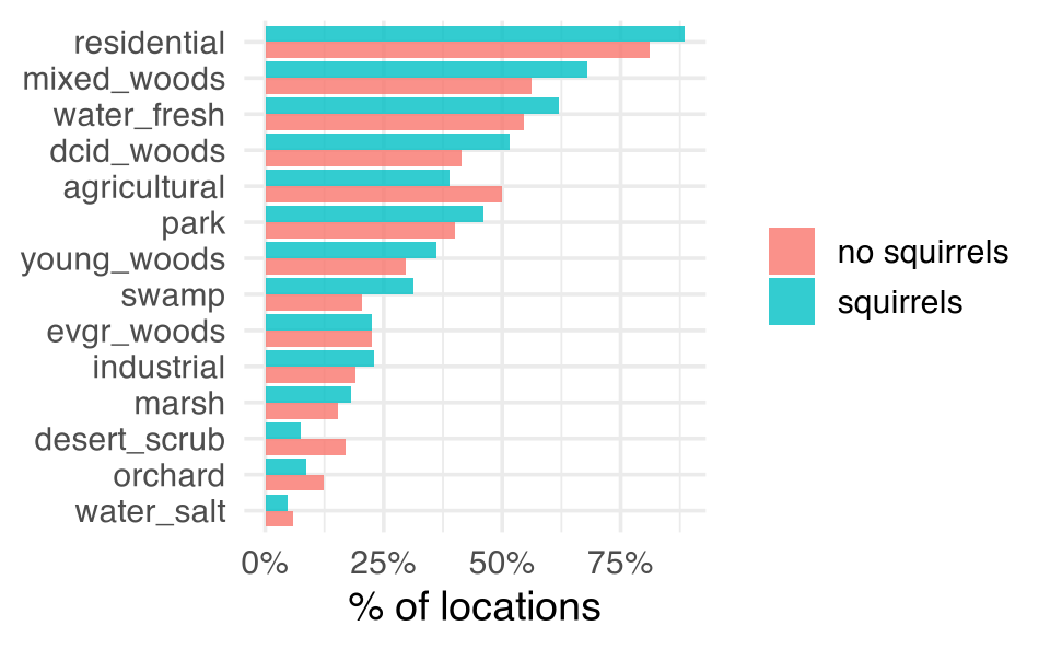

7.3 Building a Model

If the idea is to build a model which can predict squirrel activity, we need to have a way to see how we did (at the end). Indeed, it is important for us to put some data in our pocket (it will be called the “test” data) which doesn’t see any of the modeling process. We’ll use the test data at the end to assess whether or not our predictions are any good.

7.3.0.1 Create the dataset

There is a little bit of work to do to use only the observations that recodered whether or not there was a squirrel and to remove a few variables which are not of interest.

library(tidymodels)

site_data <- site_data %>%
  filter(!is.na(squirrels)) %>%
  select(where(~!all(is.na(.x)))) %>%
  select(-loc_id, -proj_period_id, -fed_yr_round) %>%
  select(squirrels, everything())

Train / test

Step 1: Create an initial split:

set.seed(470)
feeder_split <- site_data %>%
  initial_split(strata = squirrels) # prop = 3/4 in each group, by default

Step 2: Save training data

feeder_train <- training(feeder_split)
dim(feeder_train)
#> [1] 176763     59

Step 3: Save testing data

feeder_test  <- testing(feeder_split)
dim(feeder_test)
#> [1] 58922    59

Using the training data

feeder_train
#> # A tibble: 176,763 × 59
#>   squirrels    yard_type_pavement yard_type_garden yard_type_landsca
#>   <fct>                     <dbl>            <dbl>             <dbl>
#> 1 no squirrels                  0                0                 1
#> 2 no squirrels                  0                0                 1
#> 3 no squirrels                  0                0                 1
#> 4 no squirrels                  0                0                 1
#> 5 no squirrels                  0                0                 1
#> 6 no squirrels                  0                0                 1
#> # ℹ 176,757 more rows
#> # ℹ 55 more variables: yard_type_woods <dbl>, yard_type_desert <dbl>,
#> #   hab_dcid_woods <dbl>, hab_evgr_woods <dbl>, hab_mixed_woods <dbl>,
#> #   hab_orchard <dbl>, hab_park <dbl>, hab_water_fresh <dbl>,
#> #   hab_water_salt <dbl>, hab_residential <dbl>, hab_industrial <dbl>,
#> #   hab_agricultural <dbl>, hab_desert_scrub <dbl>, hab_young_woods <dbl>,
#> #   hab_swamp <dbl>, hab_marsh <dbl>, evgr_trees_atleast <dbl>, …

7.3.1 Modeling workflow

Ideally, the feature engineering / variable selection happens as part of the workflow. That is, part of the modeling process. That way, when the training data is used to fit the model, feature engineering happens. When the test data is used to come up with predictions, feature engineering also happens.

Create a recipe for feature engineering steps to be applied to the training data
Fit the model to the training data after these steps have been applied
Use the model estimates from the training data, predict outcomes for the test data
Evaluate the performance of the model on the test data

The process is synthesized in the following graphic from a course at Johns Hopkins, Tidyverse Skills for Data Science.

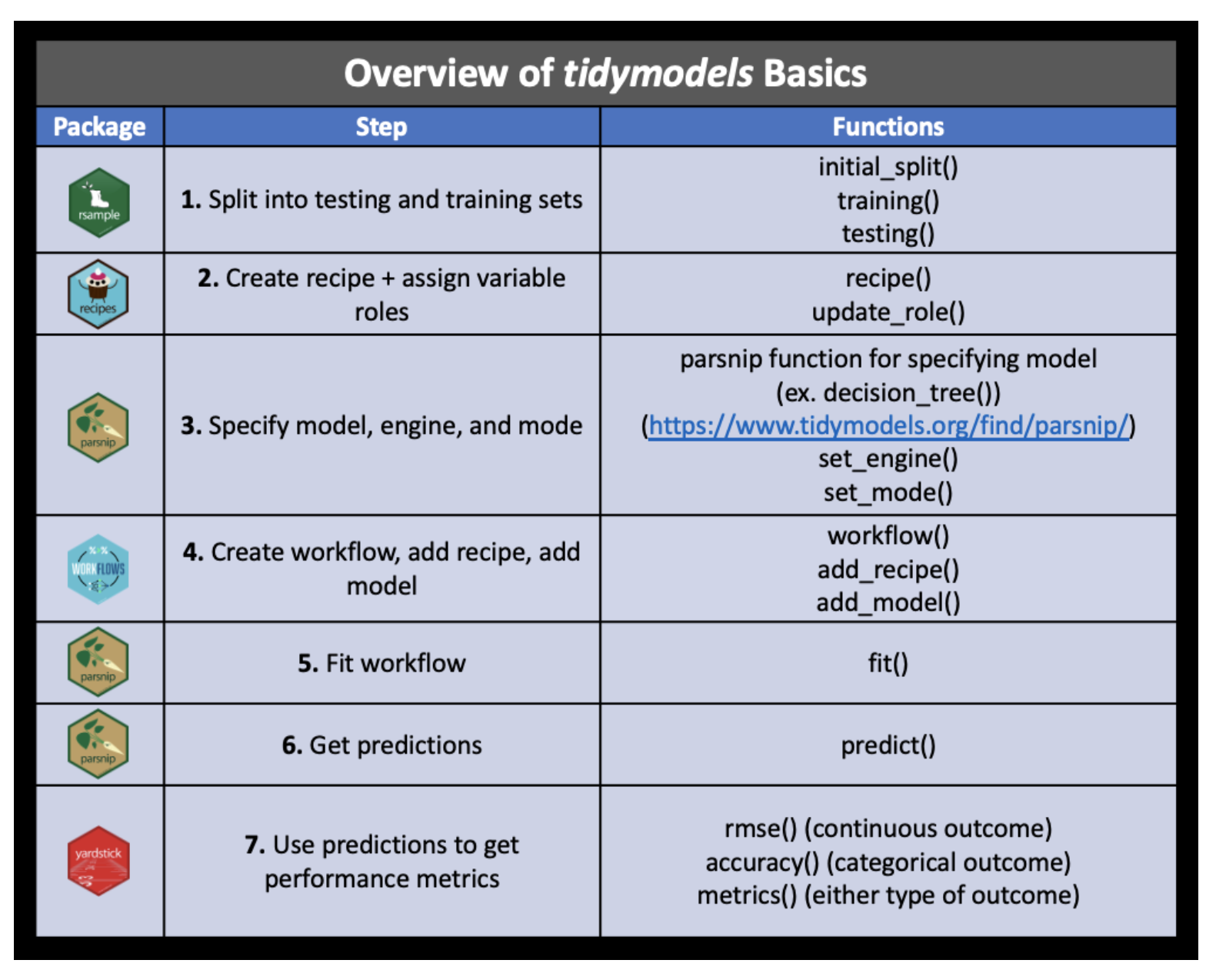
Figure 7.1: Image credit: Wright et al., Chapter 5 of Tidyverse Skills for Data Science https://jhudatascience.org/tidyversecourse/

7.3.2 Specifying a model

Instead of using the glm() command, we’re going to use the tidymodels framework to specify a model. In Math 150 we will always use “glm” as the engine, but if you take other applied statistics classes, you’ll use different model specifications with the same feature engineering and modeling fitting steps.

Note that (above) I pulled in all of the relevant functions from the package using library(tidymodels).

feeder_spec <- logistic_reg() %>%
  set_engine("glm") 

feeder_spec
#> Logistic Regression Model Specification (classification)
#> 
#> Computational engine: glm

7.3.3 Building a recipe

The steps in building a recipe are done sequentially so that the format of each variable is as desired for the model. As seen in Section (@ref{sec:wflow}), the recipe steps can happen in sequence using the pipe (%>%) function.

However, when you work with a single pipeline, the recipe effects on the data aren’t seen, which can be unsettling. You can look at what will happen when you ultimately apply the recipe to your data by using the functions prep() and bake().

Note: Using prep() and bake() are shown here for demonstrative purposes. They do not need to be a part of your pipeline. I do find them assuring, however, so that I can see the effects of the recipe steps as the recipe is built.

Initiate a recipe

feeder_rec <- recipe(
  squirrels ~ .,    # formula
  data = feeder_train # data for cataloging names and types of variables
  )

feeder_rec
#> Recipe
#> 
#> Inputs:
#> 
#>       role #variables
#>    outcome          1
#>  predictor         58

Remove zero variance predictors

Remove all predictors that contain only a single value. “zero variance” means that there is no variability in the entire column, literally every value is the same. Those variables won’t ever help with prediction.

step_impute_mean() fills in all the missing values using the average of that variable. step_nzv() creates a specification of a recipe step that will remove variables that contain only a single value.

feeder_rec <- feeder_rec %>%
  step_impute_mean(all_numeric_predictors()) %>%
  step_nzv(all_numeric_predictors())

feeder_rec
#> Recipe
#> 
#> Inputs:
#> 
#>       role #variables
#>    outcome          1
#>  predictor         58
#> 
#> Operations:
#> 
#> Mean imputation for all_numeric_predictors()
#> Sparse, unbalanced variable filter on all_numeric_predictors()

feeder_rec_trained <- prep(feeder_rec)

bake(feeder_rec_trained, feeder_train) %>%
  glimpse
#> Rows: 176,763
#> Columns: 59
#> $ yard_type_pavement           <dbl> 0, 0, 0, 0, 0, 0, 0, 0, 0, 0, 0, 0, 0, 0,…
#> $ yard_type_garden             <dbl> 0, 0, 0, 0, 0, 0, 0, 0, 0, 0, 0, 0, 0, 0,…
#> $ yard_type_landsca            <dbl> 1, 1, 1, 1, 1, 1, 0, 1, 1, 1, 1, 1, 1, 1,…
#> $ yard_type_woods              <dbl> 0, 0, 0, 0, 1, 0, 1, 1, 0, 1, 0, 1, 1, 0,…
#> $ yard_type_desert             <dbl> 0, 0, 0, 0, 0, 0, 0, 0, 0, 0, 0, 0, 0, 0,…
#> $ hab_dcid_woods               <dbl> 1.000, 1.000, 1.000, 1.000, 1.000, 1.000,…
#> $ hab_evgr_woods               <dbl> 0.223, 0.223, 0.000, 0.223, 0.000, 0.223,…
#> $ hab_mixed_woods              <dbl> 1.000, 1.000, 1.000, 0.655, 0.000, 1.000,…
#> $ hab_orchard                  <dbl> 0.0932, 0.0932, 0.0000, 0.0932, 0.0000, 0…
#> $ hab_park                     <dbl> 0.45, 0.45, 0.00, 0.45, 0.00, 0.45, 0.00,…
#> $ hab_water_fresh              <dbl> 1.000, 1.000, 1.000, 1.000, 1.000, 0.605,…
#> $ hab_water_salt               <dbl> 0.0502, 0.0502, 0.0000, 0.0502, 0.0000, 0…
#> $ hab_residential              <dbl> 1.000, 1.000, 1.000, 1.000, 1.000, 1.000,…
#> $ hab_industrial               <dbl> 0.222, 0.222, 0.000, 0.222, 0.000, 0.222,…
#> $ hab_agricultural             <dbl> 1.00, 1.00, 1.00, 0.41, 1.00, 0.41, 0.00,…
#> $ hab_desert_scrub             <dbl> 0.0926, 0.0926, 0.0000, 0.0926, 0.0000, 0…
#> $ hab_young_woods              <dbl> 0.35, 0.35, 0.00, 0.35, 0.00, 1.00, 0.00,…
#> $ hab_swamp                    <dbl> 0.292, 0.292, 0.000, 0.292, 0.000, 0.292,…
#> $ hab_marsh                    <dbl> 1.000, 1.000, 1.000, 0.175, 0.000, 0.175,…
#> $ evgr_trees_atleast           <dbl> 11, 11, 11, 0, 11, 1, 4, 4, 4, 1, 1, 1, 1…
#> $ evgr_shrbs_atleast           <dbl> 4, 4, 1, 4, 0, 1, 4, 4, 4, 1, 0, 4, 4, 11…
#> $ dcid_trees_atleast           <dbl> 11, 11, 1, 4, 1, 4, 11, 11, 4, 1, 1, 1, 1…
#> $ dcid_shrbs_atleast           <dbl> 4, 4, 4, 1, 1, 4, 11, 11, 1, 1, 0, 4, 4, …
#> $ fru_trees_atleast            <dbl> 4.00, 4.00, 1.00, 1.00, 0.00, 0.00, 2.39,…
#> $ cacti_atleast                <dbl> 0.000, 0.000, 0.000, 0.000, 0.000, 0.000,…
#> $ brsh_piles_atleast           <dbl> 0, 0, 0, 1, 0, 0, 1, 4, 1, 0, 0, 1, 1, 1,…
#> $ water_srcs_atleast           <dbl> 1.000, 1.000, 1.000, 0.000, 0.000, 0.000,…
#> $ bird_baths_atleast           <dbl> 0, 0, 0, 1, 0, 0, 1, 1, 4, 0, 0, 0, 0, 1,…
#> $ nearby_feeders               <dbl> 1, 1, 0, 1, 0, 0, 0, 1, 1, 0, 0, 0, 0, 1,…
#> $ cats                         <dbl> 1, 1, 1, 1, 0, 0, 0, 1, 0, 1, 1, 0, 0, 0,…
#> $ dogs                         <dbl> 0, 0, 0, 1, 0, 0, 0, 1, 1, 1, 1, 1, 0, 1,…
#> $ humans                       <dbl> 0, 0, 1, 1, 1, 0, 0, 1, 1, 1, 1, 1, 1, 1,…
#> $ housing_density              <dbl> 2, 2, 2, 2, 2, 3, 1, 1, 1, 1, 2, 1, 2, 2,…
#> $ fed_in_jan                   <dbl> 1.00, 1.00, 1.00, 1.00, 1.00, 1.00, 0.00,…
#> $ fed_in_feb                   <dbl> 1.000, 1.000, 1.000, 1.000, 1.000, 1.000,…
#> $ fed_in_mar                   <dbl> 1.000, 1.000, 1.000, 1.000, 1.000, 1.000,…
#> $ fed_in_apr                   <dbl> 1.000, 1.000, 0.000, 1.000, 1.000, 0.000,…
#> $ fed_in_may                   <dbl> 0.000, 0.000, 0.000, 1.000, 1.000, 0.000,…
#> $ fed_in_jun                   <dbl> 0.000, 0.000, 0.000, 1.000, 1.000, 0.000,…
#> $ fed_in_jul                   <dbl> 0.000, 0.000, 0.000, 1.000, 1.000, 0.000,…
#> $ fed_in_aug                   <dbl> 0.000, 0.000, 0.000, 1.000, 1.000, 0.000,…
#> $ fed_in_sep                   <dbl> 0.000, 0.000, 0.000, 1.000, 1.000, 0.000,…
#> $ fed_in_oct                   <dbl> 0.000, 0.000, 0.000, 1.000, 1.000, 1.000,…
#> $ fed_in_nov                   <dbl> 1, 1, 1, 1, 1, 1, 1, 1, 1, 1, 1, 1, 1, 1,…
#> $ fed_in_dec                   <dbl> 1, 1, 1, 1, 1, 1, 1, 1, 1, 1, 1, 1, 1, 1,…
#> $ numfeeders_suet              <dbl> 1, 1, 1, 2, 1, 1, 1, 1, 3, 2, 2, 3, 4, 1,…
#> $ numfeeders_ground            <dbl> 0.00, 0.00, 1.27, 1.00, 0.00, 1.00, 1.27,…
#> $ numfeeders_hanging           <dbl> 1.00, 1.00, 2.71, 2.00, 2.71, 1.00, 2.71,…
#> $ numfeeders_platfrm           <dbl> 1.00, 1.00, 1.03, 1.03, 0.00, 0.00, 1.03,…
#> $ numfeeders_humming           <dbl> 0.000, 0.000, 0.499, 0.499, 0.000, 0.000,…
#> $ numfeeders_water             <dbl> 1.000, 1.000, 0.789, 0.789, 0.789, 0.000,…
#> $ numfeeders_thistle           <dbl> 0.00, 0.00, 1.01, 1.00, 1.01, 0.00, 1.01,…
#> $ numfeeders_fruit             <dbl> 0.000, 0.000, 0.144, 0.144, 0.000, 0.000,…
#> $ numfeeders_hopper            <dbl> 1.39, 1.39, 1.00, 1.39, 0.00, 1.39, 1.39,…
#> $ numfeeders_tube              <dbl> 2.16, 2.16, 1.00, 2.16, 2.00, 2.16, 1.00,…
#> $ numfeeders_other             <dbl> 0.604, 0.604, 0.604, 0.604, 0.000, 0.604,…
#> $ population_atleast           <dbl> 1, 1, 1, 25001, 5001, 25001, 1, 1, 1, 1, …
#> $ count_area_size_sq_m_atleast <dbl> 1.01, 1.01, 1.01, 1.01, 1.01, 1.01, 375.0…
#> $ squirrels                    <fct> no squirrels, no squirrels, no squirrels,…

step_ functions

For more information: https://recipes.tidymodels.org/reference/index.html

ls(pattern = '^step_', env = as.environment('package:recipes'))
#>  [1] "step_arrange"            "step_bagimpute"         
#>  [3] "step_bin2factor"         "step_BoxCox"            
#>  [5] "step_bs"                 "step_center"            
#>  [7] "step_classdist"          "step_corr"              
#>  [9] "step_count"              "step_cut"               
#> [11] "step_date"               "step_depth"             
#> [13] "step_discretize"         "step_dummy"             
#> [15] "step_dummy_extract"      "step_dummy_multi_choice"
#> [17] "step_factor2string"      "step_filter"            
#> [19] "step_filter_missing"     "step_geodist"           
#> [21] "step_harmonic"           "step_holiday"           
#> [23] "step_hyperbolic"         "step_ica"               
#> [25] "step_impute_bag"         "step_impute_knn"        
#> [27] "step_impute_linear"      "step_impute_lower"      
#> [29] "step_impute_mean"        "step_impute_median"     
#> [31] "step_impute_mode"        "step_impute_roll"       
#> [33] "step_indicate_na"        "step_integer"           
#> [35] "step_interact"           "step_intercept"         
#> [37] "step_inverse"            "step_invlogit"          
#> [39] "step_isomap"             "step_knnimpute"         
#> [41] "step_kpca"               "step_kpca_poly"         
#> [43] "step_kpca_rbf"           "step_lag"               
#> [45] "step_lincomb"            "step_log"               
#> [47] "step_logit"              "step_lowerimpute"       
#> [49] "step_meanimpute"         "step_medianimpute"      
#> [51] "step_modeimpute"         "step_mutate"            
#> [53] "step_mutate_at"          "step_naomit"            
#> [55] "step_nnmf"               "step_nnmf_sparse"       
#> [57] "step_normalize"          "step_novel"             
#> [59] "step_ns"                 "step_num2factor"        
#> [61] "step_nzv"                "step_ordinalscore"      
#> [63] "step_other"              "step_pca"               
#> [65] "step_percentile"         "step_pls"               
#> [67] "step_poly"               "step_poly_bernstein"    
#> [69] "step_profile"            "step_range"             
#> [71] "step_ratio"              "step_regex"             
#> [73] "step_relevel"            "step_relu"              
#> [75] "step_rename"             "step_rename_at"         
#> [77] "step_rm"                 "step_rollimpute"        
#> [79] "step_sample"             "step_scale"             
#> [81] "step_select"             "step_shuffle"           
#> [83] "step_slice"              "step_spatialsign"       
#> [85] "step_spline_b"           "step_spline_convex"     
#> [87] "step_spline_monotone"    "step_spline_natural"    
#> [89] "step_spline_nonnegative" "step_sqrt"              
#> [91] "step_string2factor"      "step_time"              
#> [93] "step_unknown"            "step_unorder"           
#> [95] "step_window"             "step_YeoJohnson"        
#> [97] "step_zv"

7.3.4 Building workflows

Workflows bring together models and recipes so that they can be easily applied to both the training and test data.

Specify model

feeder_spec <- logistic_reg() %>%
  set_engine("glm")

feeder_spec
#> Logistic Regression Model Specification (classification)
#> 
#> Computational engine: glm

The workflow: Notice that the two important parts to the workflows are the model specification and the feature engineering recipe information.

feeder_wflow <- workflow() %>%
  add_model(feeder_spec) %>%
  add_recipe(feeder_rec)

feeder_wflow
#> ══ Workflow ════════════════════════════════════════════════════════════════════
#> Preprocessor: Recipe
#> Model: logistic_reg()
#> 
#> ── Preprocessor ────────────────────────────────────────────────────────────────
#> 2 Recipe Steps
#> 
#> • step_impute_mean()
#> • step_nzv()
#> 
#> ── Model ───────────────────────────────────────────────────────────────────────
#> Logistic Regression Model Specification (classification)
#> 
#> Computational engine: glm

Fit model to training data

With the workflow in hand, the model can now be fit to the training data. Although, wow… there are so many predictors!

feeder_fit <- feeder_wflow %>%
  fit(data = feeder_train)

feeder_fit %>% tidy() %>% print(n = 21)
#> # A tibble: 59 × 5
#>    term               estimate std.error statistic   p.value
#>    <chr>                 <dbl>     <dbl>     <dbl>     <dbl>
#>  1 (Intercept)         -1.42     0.0505    -28.2   2.26e-174
#>  2 yard_type_pavement  -0.854    0.149      -5.74  9.23e-  9
#>  3 yard_type_garden    -0.175    0.0392     -4.47  7.89e-  6
#>  4 yard_type_landsca    0.168    0.0219      7.69  1.45e- 14
#>  5 yard_type_woods      0.309    0.0170     18.1   1.59e- 73
#>  6 yard_type_desert    -0.297    0.0789     -3.76  1.68e-  4
#>  7 hab_dcid_woods       0.336    0.0161     20.9   6.55e- 97
#>  8 hab_evgr_woods      -0.0797   0.0192     -4.15  3.36e-  5
#>  9 hab_mixed_woods      0.420    0.0158     26.5   3.17e-155
#> 10 hab_orchard         -0.307    0.0252    -12.2   4.00e- 34
#> 11 hab_park             0.0614   0.0192      3.20  1.36e-  3
#> 12 hab_water_fresh      0.0638   0.0157      4.07  4.79e-  5
#> 13 hab_water_salt      -0.320    0.0331     -9.67  4.03e- 22
#> 14 hab_residential      0.197    0.0208      9.51  1.88e- 21
#> 15 hab_industrial      -0.0365   0.0191     -1.91  5.61e-  2
#> 16 hab_agricultural    -0.578    0.0179    -32.3   2.87e-228
#> 17 hab_desert_scrub    -0.557    0.0240    -23.2   2.42e-119
#> 18 hab_young_woods      0.0874   0.0186      4.70  2.63e-  6
#> 19 hab_swamp            0.406    0.0223     18.2   5.54e- 74
#> 20 hab_marsh           -0.0149   0.0231     -0.644 5.20e-  1
#> 21 evgr_trees_atleast   0.0405   0.00220    18.4   1.44e- 75
#> # ℹ 38 more rows

7.3.5 Evaluate the model

Predictions for training data

Model assessment

feeder_train_pred <- predict(feeder_fit, feeder_train, type = "prob") %>%
  mutate(.pred_class = as.factor(ifelse(.pred_squirrels >=0.5,
                                        "squirrels", "no squirrels"))) %>%
  bind_cols(feeder_train %>% select(squirrels))

feeder_train_pred %>% select(squirrels, .pred_class) %>% table()
#>               .pred_class
#> squirrels      no squirrels squirrels
#>   no squirrels         3448     30544
#>   squirrels            2122    140649

rbind(roc_auc(feeder_train_pred, truth = squirrels, 
              estimate = .pred_squirrels, event_level = "second"),
      accuracy(feeder_train_pred, truth = squirrels, 
               estimate = .pred_class),
      sensitivity(feeder_train_pred, truth = squirrels, 
                  estimate = .pred_class, event_level = "second"),
      specificity(feeder_train_pred, truth = squirrels, 
                  estimate = .pred_class, event_level = "second")
)
#> # A tibble: 4 × 3
#>   .metric     .estimator .estimate
#>   <chr>       <chr>          <dbl>
#> 1 roc_auc     binary         0.720
#> 2 accuracy    binary         0.815
#> 3 sensitivity binary         0.985
#> 4 specificity binary         0.101

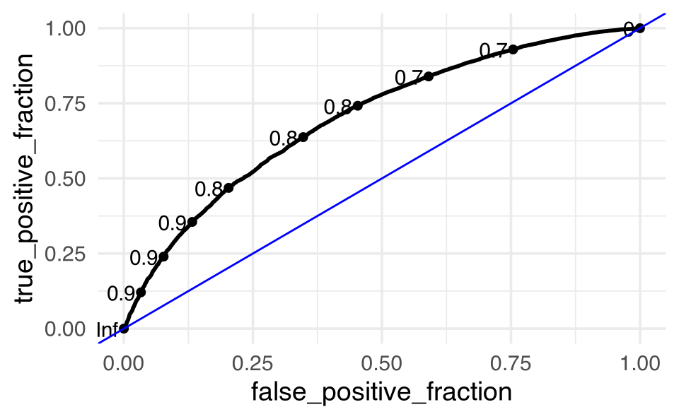
feeder_train_pred %>%
  ggplot() + 
  plotROC::geom_roc(aes(m = .pred_squirrels, d = squirrels)) + 
  geom_abline(intercept = 0, slope = 1, color = "blue")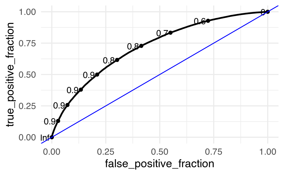

Wow, that model does TERRIBLY at predicting when there are no squirrels. Yikes! (The underlying problem is all about the imbalance in the dataset.)

But, really…

who cares about predictions on training data?

Predictions for testing data

feeder_test_pred <- predict(feeder_fit, feeder_test) %>%
  bind_cols(feeder_test %>% select(squirrels))

feeder_test_pred %>% table()
#>               squirrels
#> .pred_class    no squirrels squirrels
#>   no squirrels         1119       726
#>   squirrels           10212     46865

feeder_test_pred <- predict(feeder_fit, feeder_test, type = "prob") %>%
  mutate(.pred_class = as.factor(ifelse(.pred_squirrels >=0.5,
                                        "squirrels", "no squirrels"))) %>%
  bind_cols(feeder_test %>% select(squirrels))

feeder_test_pred %>% select(squirrels, .pred_class) %>% table()
#>               .pred_class
#> squirrels      no squirrels squirrels
#>   no squirrels         1119     10212
#>   squirrels             726     46865

rbind(roc_auc(feeder_test_pred, truth = squirrels, 
              estimate = .pred_squirrels, event_level = "second"),
      accuracy(feeder_test_pred, truth = squirrels, 
               estimate = .pred_class),
      sensitivity(feeder_test_pred, truth = squirrels, 
                  estimate = .pred_class, event_level = "second"),
      specificity(feeder_test_pred, truth = squirrels, 
                  estimate = .pred_class, event_level = "second")
)
#> # A tibble: 4 × 3
#>   .metric     .estimator .estimate
#>   <chr>       <chr>          <dbl>
#> 1 roc_auc     binary        0.721 
#> 2 accuracy    binary        0.814 
#> 3 sensitivity binary        0.985 
#> 4 specificity binary        0.0988

feeder_test_pred %>%
  ggplot() + 
  plotROC::geom_roc(aes(m = .pred_squirrels, d = squirrels)) + 
  geom_abline(intercept = 0, slope = 1, color = "blue")

Evaluating performance on training data

The training set does not have the capacity to be a good arbiter of performance.
It is not an independent piece of information; predicting the training set can only reflect what the model already knows.
Suppose you give a class a test, then give them the answers, then provide the same test. The student scores on the second test do not accurately reflect what they know about the subject; these scores would probably be higher than their results on the first test.

7.4 Cross Validation

Before reading the notes, look through this great visualization. Don’t worry about building the model (classification trees are not a topic for class), but check out the end where they talk about predicting on test and training data.

In order to motivate cross validation, let’s set up the scenario for when we need cross validation. Recall that we use the test data to assess how the model does. But we haven’t yet thought about how to use the data to build a particular model.

For example, let’s set up a scenario to compare two different models to predict whether or not there are squirrels. The first model removes the information about the habitat and about the trees and shrubs, but it is otherwise similar to the model above. The second model does use the habitat + trees + shrubs information, but it removes the information about feeding the birds.

Model 1:

feeder_rec1 <- recipe(squirrels ~ ., data = feeder_train) %>%
  # delete the habitat variables
  step_rm(contains("hab")) %>%
  # delete the tree/shrub info
  step_rm(contains("atleast")) %>%
  step_impute_mean(all_numeric_predictors()) %>%
  step_nzv(all_numeric_predictors())

prep(feeder_rec1) %>%
bake(feeder_train) %>%
  glimpse()
#> Rows: 176,763
#> Columns: 34
#> $ yard_type_pavement <dbl> 0, 0, 0, 0, 0, 0, 0, 0, 0, 0, 0, 0, 0, 0, 0, 0, 0, …
#> $ yard_type_garden   <dbl> 0, 0, 0, 0, 0, 0, 0, 0, 0, 0, 0, 0, 0, 0, 0, 0, 0, …
#> $ yard_type_landsca  <dbl> 1, 1, 1, 1, 1, 1, 0, 1, 1, 1, 1, 1, 1, 1, 1, 1, 1, …
#> $ yard_type_woods    <dbl> 0, 0, 0, 0, 1, 0, 1, 1, 0, 1, 0, 1, 1, 0, 1, 1, 1, …
#> $ yard_type_desert   <dbl> 0, 0, 0, 0, 0, 0, 0, 0, 0, 0, 0, 0, 0, 0, 0, 0, 0, …
#> $ nearby_feeders     <dbl> 1, 1, 0, 1, 0, 0, 0, 1, 1, 0, 0, 0, 0, 1, 1, 1, 1, …
#> $ cats               <dbl> 1, 1, 1, 1, 0, 0, 0, 1, 0, 1, 1, 0, 0, 0, 0, 1, 1, …
#> $ dogs               <dbl> 0, 0, 0, 1, 0, 0, 0, 1, 1, 1, 1, 1, 0, 1, 1, 1, 0, …
#> $ humans             <dbl> 0, 0, 1, 1, 1, 0, 0, 1, 1, 1, 1, 1, 1, 1, 1, 1, 0, …
#> $ housing_density    <dbl> 2, 2, 2, 2, 2, 3, 1, 1, 1, 1, 2, 1, 2, 2, 3, 3, 3, …
#> $ fed_in_jan         <dbl> 1.00, 1.00, 1.00, 1.00, 1.00, 1.00, 0.00, 1.00, 1.0…
#> $ fed_in_feb         <dbl> 1.000, 1.000, 1.000, 1.000, 1.000, 1.000, 0.000, 1.…
#> $ fed_in_mar         <dbl> 1.000, 1.000, 1.000, 1.000, 1.000, 1.000, 0.000, 1.…
#> $ fed_in_apr         <dbl> 1.000, 1.000, 0.000, 1.000, 1.000, 0.000, 0.000, 1.…
#> $ fed_in_may         <dbl> 0.000, 0.000, 0.000, 1.000, 1.000, 0.000, 0.000, 1.…
#> $ fed_in_jun         <dbl> 0.000, 0.000, 0.000, 1.000, 1.000, 0.000, 0.000, 1.…
#> $ fed_in_jul         <dbl> 0.000, 0.000, 0.000, 1.000, 1.000, 0.000, 1.000, 1.…
#> $ fed_in_aug         <dbl> 0.000, 0.000, 0.000, 1.000, 1.000, 0.000, 1.000, 1.…
#> $ fed_in_sep         <dbl> 0.000, 0.000, 0.000, 1.000, 1.000, 0.000, 1.000, 1.…
#> $ fed_in_oct         <dbl> 0.000, 0.000, 0.000, 1.000, 1.000, 1.000, 1.000, 1.…
#> $ fed_in_nov         <dbl> 1, 1, 1, 1, 1, 1, 1, 1, 1, 1, 1, 1, 1, 1, 1, 1, 1, …
#> $ fed_in_dec         <dbl> 1, 1, 1, 1, 1, 1, 1, 1, 1, 1, 1, 1, 1, 1, 1, 1, 1, …
#> $ numfeeders_suet    <dbl> 1, 1, 1, 2, 1, 1, 1, 1, 3, 2, 2, 3, 4, 1, 1, 1, 1, …
#> $ numfeeders_ground  <dbl> 0.00, 0.00, 1.27, 1.00, 0.00, 1.00, 1.27, 1.00, 0.0…
#> $ numfeeders_hanging <dbl> 1.00, 1.00, 2.71, 2.00, 2.71, 1.00, 2.71, 2.00, 3.0…
#> $ numfeeders_platfrm <dbl> 1.00, 1.00, 1.03, 1.03, 0.00, 0.00, 1.03, 2.00, 0.0…
#> $ numfeeders_humming <dbl> 0.000, 0.000, 0.499, 0.499, 0.000, 0.000, 1.000, 0.…
#> $ numfeeders_water   <dbl> 1.000, 1.000, 0.789, 0.789, 0.789, 0.000, 0.789, 1.…
#> $ numfeeders_thistle <dbl> 0.00, 0.00, 1.01, 1.00, 1.01, 0.00, 1.01, 1.00, 1.0…
#> $ numfeeders_fruit   <dbl> 0.000, 0.000, 0.144, 0.144, 0.000, 0.000, 0.144, 0.…
#> $ numfeeders_hopper  <dbl> 1.39, 1.39, 1.00, 1.39, 0.00, 1.39, 1.39, 1.39, 1.3…
#> $ numfeeders_tube    <dbl> 2.16, 2.16, 1.00, 2.16, 2.00, 2.16, 1.00, 2.16, 2.1…
#> $ numfeeders_other   <dbl> 0.604, 0.604, 0.604, 0.604, 0.000, 0.604, 0.604, 0.…
#> $ squirrels          <fct> no squirrels, no squirrels, no squirrels, no squirr…

Model 2:

feeder_rec2 <- recipe(squirrels ~ ., data = feeder_train) %>%
  # delete the variables on when the birds were fed
  step_rm(contains("fed")) %>%
  # delete the variables about the bird feeders
  step_rm(contains("feed")) %>%
  step_impute_mean(all_numeric_predictors()) %>%
  step_nzv(all_numeric_predictors())

prep(feeder_rec2) %>%
bake(feeder_train) %>%
  glimpse()
#> Rows: 176,763
#> Columns: 35
#> $ yard_type_pavement           <dbl> 0, 0, 0, 0, 0, 0, 0, 0, 0, 0, 0, 0, 0, 0,…
#> $ yard_type_garden             <dbl> 0, 0, 0, 0, 0, 0, 0, 0, 0, 0, 0, 0, 0, 0,…
#> $ yard_type_landsca            <dbl> 1, 1, 1, 1, 1, 1, 0, 1, 1, 1, 1, 1, 1, 1,…
#> $ yard_type_woods              <dbl> 0, 0, 0, 0, 1, 0, 1, 1, 0, 1, 0, 1, 1, 0,…
#> $ yard_type_desert             <dbl> 0, 0, 0, 0, 0, 0, 0, 0, 0, 0, 0, 0, 0, 0,…
#> $ hab_dcid_woods               <dbl> 1.000, 1.000, 1.000, 1.000, 1.000, 1.000,…
#> $ hab_evgr_woods               <dbl> 0.223, 0.223, 0.000, 0.223, 0.000, 0.223,…
#> $ hab_mixed_woods              <dbl> 1.000, 1.000, 1.000, 0.655, 0.000, 1.000,…
#> $ hab_orchard                  <dbl> 0.0932, 0.0932, 0.0000, 0.0932, 0.0000, 0…
#> $ hab_park                     <dbl> 0.45, 0.45, 0.00, 0.45, 0.00, 0.45, 0.00,…
#> $ hab_water_fresh              <dbl> 1.000, 1.000, 1.000, 1.000, 1.000, 0.605,…
#> $ hab_water_salt               <dbl> 0.0502, 0.0502, 0.0000, 0.0502, 0.0000, 0…
#> $ hab_residential              <dbl> 1.000, 1.000, 1.000, 1.000, 1.000, 1.000,…
#> $ hab_industrial               <dbl> 0.222, 0.222, 0.000, 0.222, 0.000, 0.222,…
#> $ hab_agricultural             <dbl> 1.00, 1.00, 1.00, 0.41, 1.00, 0.41, 0.00,…
#> $ hab_desert_scrub             <dbl> 0.0926, 0.0926, 0.0000, 0.0926, 0.0000, 0…
#> $ hab_young_woods              <dbl> 0.35, 0.35, 0.00, 0.35, 0.00, 1.00, 0.00,…
#> $ hab_swamp                    <dbl> 0.292, 0.292, 0.000, 0.292, 0.000, 0.292,…
#> $ hab_marsh                    <dbl> 1.000, 1.000, 1.000, 0.175, 0.000, 0.175,…
#> $ evgr_trees_atleast           <dbl> 11, 11, 11, 0, 11, 1, 4, 4, 4, 1, 1, 1, 1…
#> $ evgr_shrbs_atleast           <dbl> 4, 4, 1, 4, 0, 1, 4, 4, 4, 1, 0, 4, 4, 11…
#> $ dcid_trees_atleast           <dbl> 11, 11, 1, 4, 1, 4, 11, 11, 4, 1, 1, 1, 1…
#> $ dcid_shrbs_atleast           <dbl> 4, 4, 4, 1, 1, 4, 11, 11, 1, 1, 0, 4, 4, …
#> $ fru_trees_atleast            <dbl> 4.00, 4.00, 1.00, 1.00, 0.00, 0.00, 2.39,…
#> $ cacti_atleast                <dbl> 0.000, 0.000, 0.000, 0.000, 0.000, 0.000,…
#> $ brsh_piles_atleast           <dbl> 0, 0, 0, 1, 0, 0, 1, 4, 1, 0, 0, 1, 1, 1,…
#> $ water_srcs_atleast           <dbl> 1.000, 1.000, 1.000, 0.000, 0.000, 0.000,…
#> $ bird_baths_atleast           <dbl> 0, 0, 0, 1, 0, 0, 1, 1, 4, 0, 0, 0, 0, 1,…
#> $ cats                         <dbl> 1, 1, 1, 1, 0, 0, 0, 1, 0, 1, 1, 0, 0, 0,…
#> $ dogs                         <dbl> 0, 0, 0, 1, 0, 0, 0, 1, 1, 1, 1, 1, 0, 1,…
#> $ humans                       <dbl> 0, 0, 1, 1, 1, 0, 0, 1, 1, 1, 1, 1, 1, 1,…
#> $ housing_density              <dbl> 2, 2, 2, 2, 2, 3, 1, 1, 1, 1, 2, 1, 2, 2,…
#> $ population_atleast           <dbl> 1, 1, 1, 25001, 5001, 25001, 1, 1, 1, 1, …
#> $ count_area_size_sq_m_atleast <dbl> 1.01, 1.01, 1.01, 1.01, 1.01, 1.01, 375.0…
#> $ squirrels                    <fct> no squirrels, no squirrels, no squirrels,…

Creating workflows

Using each of the separate recipes, different workflows are set up:

Model 1:

feeder_wflow1 <- workflow() %>%
  add_model(feeder_spec) %>%
  add_recipe(feeder_rec1)

feeder_wflow1
#> ══ Workflow ════════════════════════════════════════════════════════════════════
#> Preprocessor: Recipe
#> Model: logistic_reg()
#> 
#> ── Preprocessor ────────────────────────────────────────────────────────────────
#> 4 Recipe Steps
#> 
#> • step_rm()
#> • step_rm()
#> • step_impute_mean()
#> • step_nzv()
#> 
#> ── Model ───────────────────────────────────────────────────────────────────────
#> Logistic Regression Model Specification (classification)
#> 
#> Computational engine: glm

Model 2:

feeder_wflow2 <- workflow() %>%
  add_model(feeder_spec) %>%
  add_recipe(feeder_rec2) 

feeder_wflow2
#> ══ Workflow ════════════════════════════════════════════════════════════════════
#> Preprocessor: Recipe
#> Model: logistic_reg()
#> 
#> ── Preprocessor ────────────────────────────────────────────────────────────────
#> 4 Recipe Steps
#> 
#> • step_rm()
#> • step_rm()
#> • step_impute_mean()
#> • step_nzv()
#> 
#> ── Model ───────────────────────────────────────────────────────────────────────
#> Logistic Regression Model Specification (classification)
#> 
#> Computational engine: glm

Fit the models to the training data

WAIT, not so fast!

Implementing Cross Validation

Figure 7.2: (Flach 2012)

Cross validation is typically used in two ways.

To assess a model’s accuracy (model assessment).
To build a model (model selection).

7.4.1 Different ways to CV

Suppose that we build a classifier on a given data set. We’d like to know how well the model classifies observations, but if we test on the samples at hand, the error rate will be much lower than the model’s inherent accuracy rate. Instead, we’d like to predict new observations that were not used to create the model. There are various ways of creating test or validation sets of data:

one training set, one test set [two drawbacks: estimate of error is highly variable because it depends on which points go into the training set; and because the training data set is smaller than the full data set, the error rate is biased in such a way that it overestimates the actual error rate of the modeling technique.]
leave one out cross validation (LOOCV)

remove one observation
build the model using the remaining n-1 points
predict class membership for the observation which was removed
repeat by removing each observation one at a time

\(V\)-fold cross validation (\(V\)-fold CV)
- like LOOCV except that the algorithm is run \(V\) times on each group (of approximately equal size) from a partition of the data set.]
- LOOCV is a special case of \(V\)-fold CV with \(V=n\)
- advantage of \(V\)-fold is computational
- \(V\)-fold often has a better bias-variance trade-off [bias is lower with LOOCV. however, because LOOCV predicts \(n\) observations from \(n\) models which are basically the same, the variability will be higher (i.e., based on the \(n\) data values). with \(V\)-fold, prediction is on \(n\) values from \(V\) models which are much less correlated. the effect is to average out the predicted values in such a way that there will be less variability from data set to data set.]

CV for Model assessment 10-fold

assume variables are set
remove 10% of the data
build the model using the remaining 90%
predict response for the 10% of the observations which were removed
repeat by removing each decile one at a time
a good measure of the model’s ability to predict is the error rate associated with the predictions on the data which have been independently predicted

CV for Model selection 10-fold

set the variables
build the model using the variables set above:
1. remove 10% of the data
2. build the model using the remaining 90%
3. predict response for the 10% of the observations which were removed
4. repeat by removing each decile one at a time
measure the CV prediction error for the \(k\) value at hand
repeat steps 1-3 and choose the variables for which the prediction error is lowest

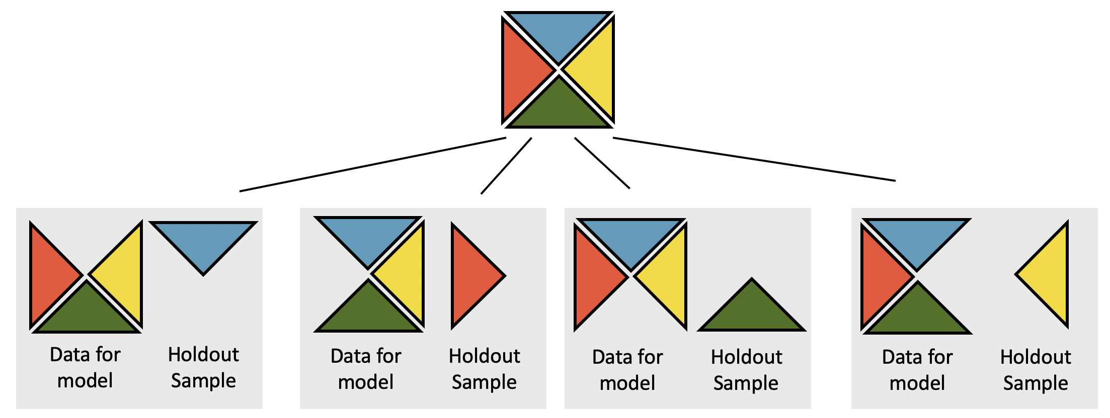
Figure 7.3: 4-fold CV is depicted. Notice that the holdout group is never used as part of the coefficient estimation process.

Once the model has been built (i.e., the variables have been selected), we can come up with a good estimate of the accuracy in the wild by applying the model to the test data.

Nested cross-validation: two cross-validation loops are run one inside the other. [@CVpaper]

Figure 7.4: Nested cross-validation: two cross-validation loops are run one inside the other. (Varoquaux et al. 2017)

7.4.2 Fit the models using cross validation

“Spending” the data

We have already established that the idea of data spending where the test set was recommended for obtaining an unbiased estimate of performance.
However, we need to decide which model to choose before using the test set.
Typically we can’t decide on which final model to take to the test set without making model assessments.
Remedy: Cross validation to make model assessments on training data in a way that can generalize to new data.

CV for model assessment

Cross validation is only conducted on the training set. The test set is not involved. For each iteration, the data are partitioned into two subsamples:

The model is fit with the analysis set.
The model is evaluated with the assessment set.

Cross validation

More specifically, v-fold cross validation:

Randomly split the training data into v partitions
Use 1 partition for assessment, and the remaining v-1 partitions for analysis
Repeat v times, updating which partition is used for assessment each time

Let’s give an example where v = 3…

Cross validation, step 1

Consider the example below where the training data are randomly split into 3 partitions:

Thirty observations are seen where three colors are used to demonstrate that the observations can be partitioned into three groups.

Figure 7.5: Splitting the data into a partition of v=3 groups. Source: (Kuhn and Silge 2022)

set.seed(4747)
folds <- vfold_cv(feeder_train, v = 3, strata = squirrels)
folds
#> #  3-fold cross-validation using stratification 
#> # A tibble: 3 × 2
#>   splits                 id   
#>   <list>                 <chr>
#> 1 <split [117841/58922]> Fold1
#> 2 <split [117842/58921]> Fold2
#> 3 <split [117843/58920]> Fold3

Note that the three repeated samples (“resamples”) are taken without replacement from the original dataset.

Cross validation, steps 2 and 3

Use 1 partition for assessment, and the remaining v-1 partitions for analysis
Repeat v times, updating which partition is used for assessment each time

Three iterations of model fitting are shown, each time using only 2/3 of the observations. The remaining 1/3 of the observations are used to estimate the performance of the model.

Figure 7.6: With the data split into three groups, we can see how 2/3 of the observations are used to fit the model and 1/3 of the observations are used to estimate the performance of the model. Source: (Kuhn and Silge 2022)

Fit CV folds

After the data have been split into v (here 3) resamples, they can each be fit to the two models of interest.

Let’s also make sure that we can get back all of the metrics we are interested in:

metrics_interest <- metric_set(accuracy, roc_auc, 
                              sensitivity, specificity)

sensitivty = number of squirrels that are accurately predicted to be squirrels (true positive rate)

specificity = number of non-squirrels that are accurately predicted to be non-squirrels (true negative rate)

feeder_train %>% select(squirrels) %>% table()
#> squirrels
#> no squirrels    squirrels 
#>        33992       142771

Model 1:

feeder_fit_rs1 <- feeder_wflow1 %>%
  fit_resamples(resamples = folds,
                metrics = metrics_interest,
                control = control_resamples(save_pred = TRUE,
                                            event_level = "second"))

feeder_fit_rs1
#> # Resampling results
#> # 3-fold cross-validation using stratification 
#> # A tibble: 3 × 5
#>   splits                 id    .metrics         .notes           .predictions
#>   <list>                 <chr> <list>           <list>           <list>      
#> 1 <split [117841/58922]> Fold1 <tibble [4 × 4]> <tibble [0 × 3]> <tibble>    
#> 2 <split [117842/58921]> Fold2 <tibble [4 × 4]> <tibble [0 × 3]> <tibble>    
#> 3 <split [117843/58920]> Fold3 <tibble [4 × 4]> <tibble [0 × 3]> <tibble>

Model 2:

feeder_fit_rs2 <- feeder_wflow2 %>%
  fit_resamples(resamples = folds,
                metrics = metrics_interest,
                control = control_resamples(save_pred = TRUE,
                                            event_level = "second"))

feeder_fit_rs2
#> # Resampling results
#> # 3-fold cross-validation using stratification 
#> # A tibble: 3 × 5
#>   splits                 id    .metrics         .notes           .predictions
#>   <list>                 <chr> <list>           <list>           <list>      
#> 1 <split [117841/58922]> Fold1 <tibble [4 × 4]> <tibble [0 × 3]> <tibble>    
#> 2 <split [117842/58921]> Fold2 <tibble [4 × 4]> <tibble [0 × 3]> <tibble>    
#> 3 <split [117843/58920]> Fold3 <tibble [4 × 4]> <tibble [0 × 3]> <tibble>

Cross validation, now what?

We’ve fit a bunch of models
Now it’s time to use them to collect metrics (e.g., accuracy or AUC) on each model and use them to evaluate model fit and how it varies across folds

Collect CV metrics

Model 1:

collect_metrics(feeder_fit_rs1)
#> # A tibble: 4 × 6
#>   .metric     .estimator   mean     n  std_err .config             
#>   <chr>       <chr>       <dbl> <int>    <dbl> <chr>               
#> 1 accuracy    binary     0.809      3 0.000247 Preprocessor1_Model1
#> 2 roc_auc     binary     0.663      3 0.00180  Preprocessor1_Model1
#> 3 sensitivity binary     0.996      3 0.000190 Preprocessor1_Model1
#> 4 specificity binary     0.0265     3 0.000545 Preprocessor1_Model1

feeder_fit_rs1 %>% augment() %>%
  select(squirrels, .pred_class) %>%
  yardstick::conf_mat(squirrels, .pred_class) %>%
  autoplot(type = "heatmap") + 
  scale_fill_gradient(low="#D6EAF8", high="#2E86C1")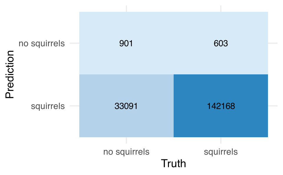

Model 2:

collect_metrics(feeder_fit_rs2)
#> # A tibble: 4 × 6
#>   .metric     .estimator   mean     n  std_err .config             
#>   <chr>       <chr>       <dbl> <int>    <dbl> <chr>               
#> 1 accuracy    binary     0.813      3 0.000325 Preprocessor1_Model1
#> 2 roc_auc     binary     0.698      3 0.00228  Preprocessor1_Model1
#> 3 sensitivity binary     0.990      3 0.000424 Preprocessor1_Model1
#> 4 specificity binary     0.0693     3 0.000291 Preprocessor1_Model1

feeder_fit_rs2 %>% augment() %>%
  select(squirrels, .pred_class) %>%
  yardstick::conf_mat(squirrels, .pred_class) %>%
  autoplot(type = "heatmap") + 
  scale_fill_gradient(low="#D6EAF8", high="#2E86C1")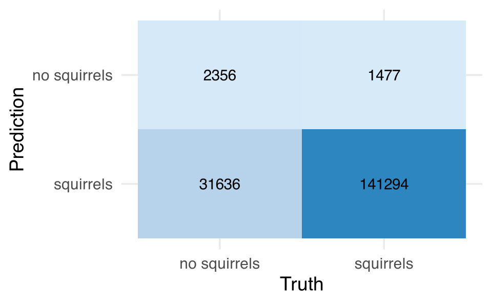

Deeper look into CV metrics

Model 1:

cv_metrics1 <- collect_metrics(feeder_fit_rs1, summarize = FALSE) 

cv_metrics1
#> # A tibble: 12 × 5
#>   id    .metric     .estimator .estimate .config             
#>   <chr> <chr>       <chr>          <dbl> <chr>               
#> 1 Fold1 accuracy    binary        0.810  Preprocessor1_Model1
#> 2 Fold1 sensitivity binary        0.996  Preprocessor1_Model1
#> 3 Fold1 specificity binary        0.0275 Preprocessor1_Model1
#> 4 Fold1 roc_auc     binary        0.666  Preprocessor1_Model1
#> 5 Fold2 accuracy    binary        0.809  Preprocessor1_Model1
#> 6 Fold2 sensitivity binary        0.995  Preprocessor1_Model1
#> # ℹ 6 more rows

Model 2:

cv_metrics2 <- collect_metrics(feeder_fit_rs2, summarize = FALSE) 

cv_metrics2
#> # A tibble: 12 × 5
#>   id    .metric     .estimator .estimate .config             
#>   <chr> <chr>       <chr>          <dbl> <chr>               
#> 1 Fold1 accuracy    binary        0.813  Preprocessor1_Model1
#> 2 Fold1 sensitivity binary        0.990  Preprocessor1_Model1
#> 3 Fold1 specificity binary        0.0687 Preprocessor1_Model1
#> 4 Fold1 roc_auc     binary        0.699  Preprocessor1_Model1
#> 5 Fold2 accuracy    binary        0.812  Preprocessor1_Model1
#> 6 Fold2 sensitivity binary        0.989  Preprocessor1_Model1
#> # ℹ 6 more rows

Better tabulation of CV metrics

Model 1:

#> # A tibble: 3 × 5
#>   id    accuracy sensitivity specificity roc_auc
#>   <chr>    <dbl>       <dbl>       <dbl>   <dbl>
#> 1 Fold1    0.81        0.996       0.028   0.666
#> 2 Fold2    0.809       0.995       0.026   0.662
#> 3 Fold3    0.809       0.996       0.026   0.66

Model 2:

#> # A tibble: 3 × 5
#>   id    accuracy sensitivity specificity roc_auc
#>   <chr>    <dbl>       <dbl>       <dbl>   <dbl>
#> 1 Fold1    0.813       0.99        0.069   0.699
#> 2 Fold2    0.812       0.989       0.069   0.701
#> 3 Fold3    0.813       0.99        0.07    0.693

Conclusions:

The logistic model is terrible at predicting when there are no squirrels (this is partly due to imbalanced data).
It seems as though the linear model which includes the information about the habitat and the trees does a slightly better job than the linear model that includes the information about when and how the birds are fed.

Cross validation jargon

Referred to as v-fold or k-fold cross validation
Also commonly abbreviated as CV

Cross validation, redux

To illustrate how CV works, we used v = 3:
Analysis sets are 2/3 of the training set
Each assessment set is a distinct 1/3
The final resampling estimate of performance averages each of the 3 replicates
It was useful for illustrative purposes, but v = 3 is a poor choice in practice
Values of v are most often 5 or 10; we generally prefer 10-fold cross-validation as a default

7.5 Final model assessment

Now that Model 2 has been chosen as the better model, the test data is finally brought in to measure how well Model 2 will predict data in the wild.

Model 2:

n.b. For whatever reason, collect_metrics() only works when multiple models have been run. When a single model is run, the metrics need to be evaluated individually.

feeder_preds2 <- feeder_wflow2 %>%
  fit(data = feeder_train) %>%
  predict(feeder_test, type = "prob") %>% 
  mutate(.pred_class = as.factor(ifelse(.pred_squirrels >=0.5,
                              "squirrels", "no squirrels"))) %>%
  bind_cols(feeder_test %>% select(squirrels)) 

rbind(roc_auc(feeder_preds2, truth = squirrels, 
              estimate = .pred_squirrels, event_level = "second"),
      accuracy(feeder_preds2, truth = squirrels, 
               estimate = .pred_class, event_level = "second"),
      sensitivity(feeder_preds2, truth = squirrels, 
                  estimate = .pred_class, event_level = "second"),
      specificity(feeder_preds2, truth = squirrels, 
                  estimate = .pred_class, event_level = "second")
)
#> # A tibble: 4 × 3
#>   .metric     .estimator .estimate
#>   <chr>       <chr>          <dbl>
#> 1 roc_auc     binary        0.702 
#> 2 accuracy    binary        0.813 
#> 3 sensitivity binary        0.989 
#> 4 specificity binary        0.0697

7.6 R: Full pipeline with CV + assessment

The following example uses tidymodels modeling to work through different aspects of the logistic regression model. Using the same example as above, the process has been synthesized into the essential aspects / code.

7.6.1 The data

Break the data into test and training sets.

set.seed(470)
feeder_split <- site_data %>%
  initial_split(strata = squirrels) # prop = 3/4 in each group, by default
feeder_train <- training(feeder_split)
feeder_test <- testing(feeder_split)

7.6.2 The model / enigne

Tell the computer to run logistic regression using the glm() function.

feeder_spec <- logistic_reg() %>%
  set_engine("glm")

7.6.3 The recipe(s)

Set the variables of interest (in the formula) and perform any necessary feature engineering.

feeder_rec <- recipe(
  squirrels ~ .,    # formula
  data = feeder_train # data for cataloging names and types of variables
  ) %>%
  step_impute_mean(all_numeric_predictors()) %>%
  step_nzv(all_numeric_predictors())

feeder_rec1 <- recipe(squirrels ~ ., data = feeder_train) %>%
  # delete the habitat variables
  step_rm(contains("hab")) %>%
  # delete the tree/shrub info
  step_rm(contains("atleast")) %>%
  step_impute_mean(all_numeric_predictors()) %>%
  step_nzv(all_numeric_predictors())


feeder_rec2 <- recipe(squirrels ~ ., data = feeder_train) %>%
  # delete the variables on when the birds were fed
  step_rm(contains("fed")) %>%
  # delete the variables about the bird feeders
  step_rm(contains("feed")) %>%
  step_impute_mean(all_numeric_predictors()) %>%
  step_nzv(all_numeric_predictors())

7.6.4 The workflow(s)

feeder_wflow <- workflow() %>%
  add_model(feeder_spec) %>%
  add_recipe(feeder_rec)

feeder_wflow1 <- workflow() %>%
  add_model(feeder_spec) %>%
  add_recipe(feeder_rec1)

feeder_wflow2 <- workflow() %>%
  add_model(feeder_spec) %>%
  add_recipe(feeder_rec2)

7.6.5 Choice: fit the model? cross validate to decide between models?

Fit the model

feeder_fit <- feeder_wflow %>%
  fit(data = feeder_train)

The fit object is the same as the output of glm() that you are used to working with:

feeder_fit %>% tidy()
#> # A tibble: 59 × 5
#>   term               estimate std.error statistic   p.value
#>   <chr>                 <dbl>     <dbl>     <dbl>     <dbl>
#> 1 (Intercept)          -1.42     0.0505    -28.2  2.26e-174
#> 2 yard_type_pavement   -0.854    0.149      -5.74 9.23e-  9
#> 3 yard_type_garden     -0.175    0.0392     -4.47 7.89e-  6
#> 4 yard_type_landsca     0.168    0.0219      7.69 1.45e- 14
#> 5 yard_type_woods       0.309    0.0170     18.1  1.59e- 73
#> 6 yard_type_desert     -0.297    0.0789     -3.76 1.68e-  4
#> # ℹ 53 more rows

feeder_fit %>% glance()
#> # A tibble: 1 × 8
#>   null.deviance df.null  logLik     AIC     BIC deviance df.residual   nobs
#>           <dbl>   <int>   <dbl>   <dbl>   <dbl>    <dbl>       <int>  <int>
#> 1       173067.  176762 -77659. 155435. 156030.  155317.      176704 176763

Cross validate to choose between models

If cross validating, the model needs to be fit separately on each one of the hold out folds of the CV model. Here, v=10 is used, different from above where v=3 was used to simplify the explanation. Typically, the number of folds is 5 or 10.

Note that the objects are now similar to what you’ve worked with previously (output of glm()), but they contain a separate fit (i.e., linear model) for each of the CV folds.

set.seed(47)
folds <- vfold_cv(feeder_train, v = 10)

feeder_fit_rs1 <- feeder_wflow1 %>%
  fit_resamples(folds,
                metrics = metrics_interest,
                control = control_resamples(save_pred = TRUE,
                                            event_level = "second"))

feeder_fit_rs2 <- feeder_wflow2 %>%
  fit_resamples(folds,
                metrics = metrics_interest,
                control = control_resamples(save_pred = TRUE,
                                            event_level = "second"))

7.6.6 Assess the fit

On the test data

Note that we should only assess the fit to the test data if we are done with the model building process and we’ve chosen the model we want to move forward with.

Accuracy, AUC, sensitivity, and specificity are all calculated.

If the first few lines don’t make sense, run the pieces. That is, run predict(feeder_fit, feeder_test) and then run feeder_test %>% select(imdb_rating, title) and then think about what it would mean to bind those columns together.

feeder_test_pred <- predict(feeder_fit, feeder_test, type = "prob") %>%
  mutate(.pred_class = as.factor(ifelse(.pred_squirrels >=0.5,
                                        "squirrels", "no squirrels"))) %>%
  bind_cols(feeder_test %>% select(squirrels))

rbind(roc_auc(feeder_test_pred, truth = squirrels, 
              estimate = .pred_squirrels, event_level = "second"),
      accuracy(feeder_test_pred, truth = squirrels, 
               estimate = .pred_class),
      sensitivity(feeder_test_pred, truth = squirrels, 
                  estimate = .pred_class, event_level = "second"),
      specificity(feeder_test_pred, truth = squirrels, 
                  estimate = .pred_class, event_level = "second")
)
#> # A tibble: 4 × 3
#>   .metric     .estimator .estimate
#>   <chr>       <chr>          <dbl>
#> 1 roc_auc     binary        0.721 
#> 2 accuracy    binary        0.814 
#> 3 sensitivity binary        0.985 
#> 4 specificity binary        0.0988

feeder_test_pred %>%
  ggplot() + 
  plotROC::geom_roc(aes(m = .pred_squirrels, d = squirrels)) + 
  geom_abline(intercept = 0, slope = 1, color = "blue")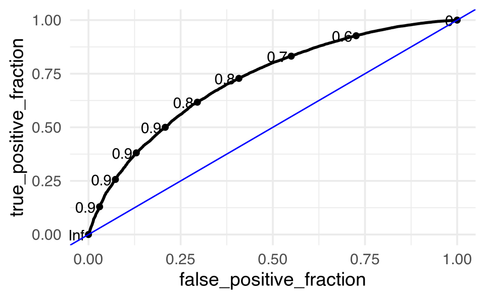

On the CV folds

Note the difference in the information. If you want the values per fold, don’t summarize. If you want the overall information, do summarize.

feeder_fit_rs1 %>% collect_metrics()
#> # A tibble: 4 × 6
#>   .metric     .estimator   mean     n  std_err .config             
#>   <chr>       <chr>       <dbl> <int>    <dbl> <chr>               
#> 1 accuracy    binary     0.810     10 0.000747 Preprocessor1_Model1
#> 2 roc_auc     binary     0.663     10 0.00183  Preprocessor1_Model1
#> 3 sensitivity binary     0.996     10 0.000154 Preprocessor1_Model1
#> 4 specificity binary     0.0269    10 0.000563 Preprocessor1_Model1
feeder_fit_rs2 %>% collect_metrics()
#> # A tibble: 4 × 6
#>   .metric     .estimator   mean     n  std_err .config             
#>   <chr>       <chr>       <dbl> <int>    <dbl> <chr>               
#> 1 accuracy    binary     0.813     10 0.000727 Preprocessor1_Model1
#> 2 roc_auc     binary     0.698     10 0.00162  Preprocessor1_Model1
#> 3 sensitivity binary     0.990     10 0.000367 Preprocessor1_Model1
#> 4 specificity binary     0.0695    10 0.00156  Preprocessor1_Model1

feeder_fit_rs1 %>% collect_metrics(summarize = FALSE)
#> # A tibble: 40 × 5
#>   id     .metric     .estimator .estimate .config             
#>   <chr>  <chr>       <chr>          <dbl> <chr>               
#> 1 Fold01 accuracy    binary        0.808  Preprocessor1_Model1
#> 2 Fold01 sensitivity binary        0.996  Preprocessor1_Model1
#> 3 Fold01 specificity binary        0.0263 Preprocessor1_Model1
#> 4 Fold01 roc_auc     binary        0.661  Preprocessor1_Model1
#> 5 Fold02 accuracy    binary        0.805  Preprocessor1_Model1
#> 6 Fold02 sensitivity binary        0.996  Preprocessor1_Model1
#> # ℹ 34 more rows
feeder_fit_rs2 %>% collect_metrics(summarize = FALSE)
#> # A tibble: 40 × 5
#>   id     .metric     .estimator .estimate .config             
#>   <chr>  <chr>       <chr>          <dbl> <chr>               
#> 1 Fold01 accuracy    binary        0.814  Preprocessor1_Model1
#> 2 Fold01 sensitivity binary        0.991  Preprocessor1_Model1
#> 3 Fold01 specificity binary        0.0738 Preprocessor1_Model1
#> 4 Fold01 roc_auc     binary        0.701  Preprocessor1_Model1
#> 5 Fold02 accuracy    binary        0.809  Preprocessor1_Model1
#> 6 Fold02 sensitivity binary        0.991  Preprocessor1_Model1
#> # ℹ 34 more rows

Note that the variables in Model 2 perform better using cross validation than the variables in Model 1, we choose Model 2 to report out:

feeder_test_pred_2 <- feeder_wflow2 %>%
  fit(feeder_train) %>%
  predict(feeder_test, type = "prob") %>%
  mutate(.pred_class = as.factor(ifelse(.pred_squirrels >=0.5,
                                        "squirrels", "no squirrels"))) %>%
  bind_cols(feeder_test %>% select(squirrels))

rbind(roc_auc(feeder_test_pred_2, truth = squirrels, 
              estimate = .pred_squirrels, event_level = "second"),
      accuracy(feeder_test_pred_2, truth = squirrels, 
               estimate = .pred_class),
      sensitivity(feeder_test_pred_2, truth = squirrels, 
                  estimate = .pred_class, event_level = "second"),
      specificity(feeder_test_pred_2, truth = squirrels, 
                  estimate = .pred_class, event_level = "second")
)
#> # A tibble: 4 × 3
#>   .metric     .estimator .estimate
#>   <chr>       <chr>          <dbl>
#> 1 roc_auc     binary        0.702 
#> 2 accuracy    binary        0.813 
#> 3 sensitivity binary        0.989 
#> 4 specificity binary        0.0697

feeder_test_pred_2 %>%
  ggplot() + 
  plotROC::geom_roc(aes(m = .pred_squirrels, d = squirrels)) + 
  geom_abline(intercept = 0, slope = 1, color = "blue")

6 Logistic Regression

8 Survival Analysis

7 Modeling as a Process

7.1 Comparing Models3

Worth a comment

Bias-variance trade-off

7.2 Modeling Squirrel Activity

7.3 Building a Model

7.3.0.1 Create the dataset

Train / test

Using the training data

7.3.1 Modeling workflow

7.3.2 Specifying a model

7.3.3 Building a recipe

Initiate a recipe

Remove zero variance predictors

7.3.4 Building workflows

Specify model

Fit model to training data

7.3.5 Evaluate the model

Predictions for training data

Model assessment

Predictions for testing data

Evaluating performance on training data

7.4 Cross Validation

Creating workflows

Fit the models to the training data

Implementing Cross Validation

7.4.1 Different ways to CV

CV for Model assessment 10-fold

CV for Model selection 10-fold

7.4.2 Fit the models using cross validation

“Spending” the data

CV for model assessment

Cross validation

Cross validation, step 1

Cross validation, steps 2 and 3

Fit CV folds

Cross validation, now what?

Collect CV metrics

Deeper look into CV metrics

Better tabulation of CV metrics

Cross validation jargon

Cross validation, redux

7.5 Final model assessment

7.6 R: Full pipeline with CV + assessment

7.6.1 The data

7.6.2 The model / enigne

7.6.3 The recipe(s)

7.6.4 The workflow(s)

7.6.5 Choice: fit the model? cross validate to decide between models?

Fit the model

Cross validate to choose between models

7.6.6 Assess the fit

On the test data

On the CV folds

7.1 Comparing Models³