4 Simple Linear Regression

Though we’ve discussed the relationship between tests of means and simple linear regression, we will really consider simple linear regression in a much broader context (one where both the explanatory and response variables are quantitative).

The data below represents 10 different variables on health of a country measured on 143 countries. Data taken from (Lock et al. 2016), originally from the Happy Planet Index Project. Region of the world is coded as 1 = Latin America, 2 = Western nations, 3 = Middle East, 4 = Sub-Saharan Africa, 5 = South Asia, 6 = East Asia, 7 = former Communist countries. We are going to investigate happiness and life expectancy.

4.1 Inference on the Linear Model

In order to make an inferential claims on a linear regression model (e.g., p-values on hypotheses about coefficients, confidence intervals for coefficients, confidence interval for the line, prediction interval for the points, …), we have a set of technical conditions that provide the mathematical structure leading to the t-procedures (e.g., t-test). A course more focused on linear regression would spend time discussing how robust the model is to various deviations from the following technical conditions. For now, we will say that sometimes transformations of either the explanatory or response variables can be an effective way to mitigate deviations from the model.

As with any measurement of the data / population, regression models are built from either statistics (Roman letters to describe a sample) or parameters (Greek letters to describe a population). For linear regression, we have one additional differentiation due to whether the observed values \((y_i)\) or the average values \((\hat{y}_i\) or \(E[Y_i])\) are being modeled.

\[\begin{eqnarray*} E[Y_i|x_i] &=& \beta_0 + \beta_1 x_i \\ y_i &=& \beta_0 + \beta_1 x_i + \epsilon_i\\ && \epsilon_i = y_i - (\beta_0 + \beta_1 x_i)\\ \hat{y}_i &=& b_0 + b_1 x_i\\ y_i &=& b_0 + b_1 x_i + e_i\\ && e_i = y_i - \hat{y}_i = y_i - (b_0 + b_1 x_i)\\ \epsilon_i &\sim& N(0, \sigma^2) \end{eqnarray*}\]

4.1.1 Technical Conditions

The average value for the response variable is a linear function of the explanatory variable.
The error terms follow a normal distribution around the linear model.
The error terms have a mean of zero.
The error terms have a constant variance of \(\sigma^2.\)
The error terms are independent (and identically distributed).
Regression applet

How do we tell whether the assumptions are met? We can’t always. But it’s good to look at plots: scatter plot, residual plot, histograms of residuals. We denote the residuals for this model as:

\[\begin{align} r_i = \hat{e}_i = y_i - \hat{y}_i \end{align}\]

Figure 1.2: Figs 3.13 and 3.15 taken from Kutner et al. (2004).

important note!! The idea behind transformations is to make the model as appropriate as possible for the data at hand. We want to find the correct linear model; we want our assumptions to hold. We are not trying to find the most significant model or big \(R^2.\)

See section 2.9 in Kuiper and Sklar (2013). No normal probability plots (qq-plots); use histograms or boxplots to assess the symmetry and normality of the residuals.

4.2 Fitting the regression line

How do we fit a regression line? Find \(b_0\) and \(b_1\) that minimize the sum of squared distance of the points to the line (called ordinary least squares):

\[\begin{align} \min \sum (y_i - \hat{y}_i)^2 &= \min RSS \mbox{ residual sum of squares}\\ RSS &= \sum (y_i - b_0 - b_1 x_i)^2\\ \frac{\partial RSS}{\partial b_0} &= 0\\ \frac{\partial RSS}{\partial b_1} &= 0\\ b_0 &= \overline{y} - b_1 \overline{x}\\ b_1 &= r \frac{s_y}{s_x}\\ &= \frac{\sum(x_i - \overline{X})(y_i - \overline{y})}{\sum(x_i - \overline{x})^2} \end{align}\]

Is that the only way to find values for \(b_0\) and \(b_1\)? (absolute distances, maximum likelihood,…)
Resistance to outliers?
What is \(\hat{y}\) at \(\overline{x}\)?

\[\begin{align} \hat{y} &= b_0 + b_1 \overline{x}\\ &= \overline{y} - b_1 \overline{x} + b_1 \overline{x}\\ &= \overline{y} \end{align}\]

The regression line will always pass through the point \((\overline{x}, \overline{y}).\)

Definition 4.1 An estimate is unbiased if, over many repeated samples drawn from the population, the average value of the estimates based on the different samples would equal the population value of the parameter being estimated. That is, a statistic is unbiased if the mean of its sampling distribution is the population parameter.

4.3 Correlation

Consider a scatterplot, you’ll have variability in both directions: \((x_i - \overline{x}) \ \ \& \ \ (y_i - \overline{y}).\)

\[\begin{align} \mbox{sample covariance}&\\ cov(x,y) &= \frac{1}{n-1}\sum (x_i - \overline{x}) (y_i - \overline{y})\\ \mbox{sample correlation}&\\ r(x,y) &= \frac{cov(x,y)}{s_x s_y}\\ &= \frac{\frac{1}{n-1} \sum (x_i - \overline{x}) (y_i - \overline{y})}{\sqrt{\frac{\sum(x_i - \overline{x})^2}{n-1} \frac{\sum(y_i - \overline{y})^2}{n-1}}}\\ \mbox{pop cov} &= \sigma_{xy}\\ \mbox{pop cor} &= \rho = \frac{\sigma_{xy}}{\sigma_x \sigma_y}\\ \end{align}\]

\(-1 \leq r \leq 1 \ \ \ \ \ \& \ \ \ -1 \leq \rho \leq 1.\)
No Spearman’s rank correlation or Kendall’s \(\tau.\)
\(b_1 = r \frac{s_y}{s_x}\)
- if \(r=0, b_1=0\)
- if \(r=1, b_1 > 0\) but can be anything!
- \(r < 0 \leftrightarrow b_1 < 0, r > 0 \leftrightarrow b_1 > 0\)
Recall that \(R^2\) is the proportion of variability explained by the line.

4.4 Errors / Residuals

Recall, part of the technical conditions required that \(\epsilon_i \sim N(0, \sigma^2).\) How do we estimate \(\sigma^2?\)

\[\begin{align} RSS &= \sum (y_i - \hat{y}_i)^2 \ \ \ \mbox{ residual sum of squares}\\ MSS &= \sum (\hat{y}_i - \overline{y})^2 \ \ \ \mbox{ model sum of squares}\\ TSS &= \sum (y_i - \overline{y})^2 \ \ \ \mbox{ total sum of squares}\\ s_{y|x}^2 &= \hat{\sigma^2} = \frac{1}{n-2} RSS\\ s_x^2 &= \frac{1}{n-1} \sum (x_i - \overline{x})^2\\ s_y^2 &= \frac{1}{n-1} \sum (y_i - \overline{y})^2\\ var(\epsilon) &= s_{y|x}^2 = \frac{RSS}{n-2} = \frac{\sum(y_i - \hat{y}_i)^2}{n-2} = SE(\epsilon)\\ var(b_1) &= \frac{s_{y|x}^2}{(n-1) s_x^2}\\ SE(b_1) &= \frac{s_{y|x}}{\sqrt{(n-1)} s_x}\\ &= \frac{\hat{\sigma}}{\sqrt{\sum(x_i - \overline{x})^2}} = \frac{\sqrt{\sum(y_i - \hat{y}_i)^2/(n-2)}}{\sqrt{\sum(x_i - \overline{x})^2}}\\ \end{align}\]

\(SE(b_1) \downarrow\) as \(\sigma \downarrow\)
\(SE(b_1) \downarrow\) as \(n \uparrow\)
\(SE(b_1) \downarrow\) as \(s_x \uparrow\)
WHY?
What do we mean by \(SE(b_1)\)?

As we saw above, the correlation and the slope estimates are intimately related. They are also both related to the coefficient of determination. \[\begin{align} R^2 = r^2 = \frac{MSS}{TSS} \end{align}\]

\(R^2\) is the proportion of total variability explained by the regression line (the linear relationship between the explanatory and response variables).

If \(x\) and \(y\) are not at all correlated, \(\hat{y}_i \approx \overline{y},\) MSS = 0, \(R^2=0.\)
If \(x\) and \(y\) are perfectly correlated, \(\hat{y}_i = y_i,\) MSS=TSS, \(R^2 = 1.\)

4.4.1 Testing \(\beta_1\)

If the technical conditions hold, the mathematics describing the sampling distribution of \(b_1\) are well defined. That is:

If \(H_0: \beta=0\) is true, then \[\begin{align} \frac{b_1 - 0}{SE(b_1)} \sim t_{n-2} \end{align}\] Note that the degrees of freedom are now \(n-2\) because we are estimating two parameters \((\beta_0\) and \(\beta_1).\) We can also find a \((1-\alpha)100\%\) confidence interval for \(\beta_1\): \[\begin{align} b_1 \pm t_{\alpha/2, n-2} SE(b_1) \end{align}\]

4.5 Intervals

As with anything that has some type of standard error, we can create intervals that give us some confidence in the statements we are making.

4.5.1 Confidence Intervals

In general, confidence intervals are of the form:

point estimate +/- multiplier * SE(point estimate)

4.5.2 Slope

We can create a CI for the slope parameter, \(\beta_1\): \[\begin{align} b_1 &\pm t_{\alpha/2,n-2} SE(b_1)\\ b_1 &\pm t_{\alpha/2, n-2} \frac{s_{y|x}}{\sqrt{(n-1)}s_x}\\ 6.693 &\pm t_{.025, 141} 0.375\\ t_{.025,141} &= qt(0.025, 141) = -1.977\\ \mbox{CI: } & (5.95 \mbox{ years/unit of happy}, 7.43 \mbox{ years/unit of happy}) \end{align}\] How can we interpret the CI? Does it make sense to talk about a unit of happiness?

4.5.3 Mean Response

We can also create a CI for the mean response, \(E[Y|x^*] = \beta_0 + \beta_1 x^*.\) Note that the standard error of the point estimate \((\hat{y}=b_0 + b_1 x^*)\) now depends on the variability associated with two things (\(b_0, b_1).\) \[\begin{align} SE(\hat{y(x^*)}) &= \sqrt{ \frac{s^2_{y|x}}{n} + (x^* - \overline{x})^2 SE(b_1)^2}\\ SE(\hat{y}(\overline{x})) &= s_{y|x}/\sqrt{n}\\ SE(\hat{y}(x)) &\geq s_{y|x}/\sqrt{n} \ \ \ \forall x \end{align}\] How would you interpret the associated interval?

4.5.4 Prediction of an Individual Response

As should be obvious, predicting an individual is more variable than predicting a mean.

\[\begin{align} SE(y(x^*)) &= \sqrt{ \frac{s^2_{y|x}}{n} + (x^* - \overline{x})^2 SE(b_1)^2 + s^2_{y|x}}\\ SE(y(x^*)) &= \sqrt{ SE(\hat{y}(x^*))^2 + s^2_{y|x}}\\ \end{align}\] How would you interpret the associated interval?

4.6 Influential Points

We are skipping Section 4.6; you are not responsible for it.

Theorem 4.1 High leverage points are x-outliers with the potential to exert undue influence on regression coefficient estimates. Influential points are points that have exerted undue influence on the regression coefficient estimates.

Note: typically we think of more data as better; more values will tend to decrease the sampling variability of our statistic. But if I give you a lot more data and put it all at \(\overline{x},\) \(SE(b_1)\) stays exactly the same. Why??

Recall \[\begin{align} y_{i} &= \beta_0 + \beta_1 x_i \ \ \ \epsilon_i \sim N(0,\sigma^2)\\ e_i &= y_i - \hat{y}_i \end{align}\]

We plot \(e_i\) versus \(\hat{y}_i.\) (Why? Typically, we want the \(e_i\) to be constant at each value of \(x_i.\) Note that \(\hat{y}_i\) is a simple linear transformation of \(x_i,\) so the plot is identical.) We want to see if the distributions of the residuals is different across the fitted line (we look for patterns).

Not all residuals have an equal effect on the regression line!!

4.6.1 leverage

\[\begin{align} h_i = \frac{1}{n} +\frac{(x_i - \overline{x})^2}{\sum_{j=1}^n (x_j - \overline{x})^2}\\ \frac{1}{n} \leq h_i \leq 1\\ \end{align}\] Leverage represents the effect of point \(x_i\) on the line. We need large leverage for a particular value to have a large effect.

Note: \[\begin{align} SE(\hat{y}(x_i)) &= s_{y|x} \sqrt{h_i}\\ SE(y(x_i)) &= s_{y|x} \sqrt{(h_i + 1)}\\ SE(e_i) &= s_{y|x} \sqrt{(1-h_i)}\\ \hat{y}(x^*) &\pm t_{n-2, .025} (s_{y|x} \sqrt{h(x^*)+1})\\ \end{align}\] is a 95% prediction interval at \(x^*.\) High leverage reduces the variability because the line gets pulled toward the point.

4.6.2 standardized residuals

\[\begin{align} \frac{e_i}{s_{y|x} \sqrt{1-h_i}} \sim t_{n-2}\\ \end{align}\]

4.6.3 studentized residuals

\[\begin{align} \frac{e_i}{s_{y|x, (i)} \sqrt{1-h_i}} &\sim t_{n-3}\\ s_{y|x, (i)} &= \frac{1}{n-3} \sum_{j \ne i} (y_j - \hat{y}_{j(i)})^2 \end{align}\]

Where do we predict 90% of residuals? \(\pm t_{n-2,3 , .05}.\) Approximately \(\pm 2.\)

4.6.4 DFBETAs

DFBETAs represent the change in the parameter estimate due to one observation.

\[\begin{align} DFBETAS_i &= \frac{b_1 - b_{1(i)}}{\frac{s_{y|x, (i)}}{\sqrt{(n-1)} s_x}}\\ \end{align}\]

4.7 R Example (SLR): Happy Planet

The data below represents 10 different variables on health of a country measured on 143 countries. Data taken from (Lock et al. 2016), originally from the Happy Planet Index Project [http://www.happyplanetindex.org/]. Region of the world is coded as 1 = Latin America, 2 = Western nations, 3 = Middle East, 4 = Sub-Saharan Africa, 5 = South Asia, 6 = East Asia, 7 = former Communist countries. We are going to investigate happiness and life expectancy.

4.7.1 Reading the data into R

happy <- read_delim("./data/happyPlanet.txt", delim="\t")
glimpse(happy)  
#> Rows: 143
#> Columns: 11
#> $ Country        <chr> "Albania", "Algeria", "Angola", "Argentina", "Armenia",…
#> $ Region         <dbl> 7, 3, 4, 1, 7, 2, 2, 7, 5, 7, 2, 1, 4, 5, 1, 7, 4, 1, 7…
#> $ Happiness      <dbl> 5.5, 5.6, 4.3, 7.1, 5.0, 7.9, 7.8, 5.3, 5.3, 5.8, 7.6, …
#> $ LifeExpectancy <dbl> 76.2, 71.7, 41.7, 74.8, 71.7, 80.9, 79.4, 67.1, 63.1, 6…
#> $ Footprint      <dbl> 2.2, 1.7, 0.9, 2.5, 1.4, 7.8, 5.0, 2.2, 0.6, 3.9, 5.1, …
#> $ HLY            <dbl> 41.7, 40.1, 17.8, 53.4, 36.1, 63.7, 61.9, 35.4, 33.1, 4…
#> $ HPI            <dbl> 47.9, 51.2, 26.8, 59.0, 48.3, 36.6, 47.7, 41.2, 54.1, 3…
#> $ HPIRank        <dbl> 54, 40, 130, 15, 48, 102, 57, 85, 31, 104, 64, 27, 134,…
#> $ GDPperCapita   <dbl> 5316, 7062, 2335, 14280, 4945, 31794, 33700, 5016, 2053…
#> $ HDI            <dbl> 0.801, 0.733, 0.446, 0.869, 0.775, 0.962, 0.948, 0.746,…
#> $ Population     <dbl> 3.15, 32.85, 16.10, 38.75, 3.02, 20.40, 8.23, 8.39, 153…

4.7.2 Running the linear model (lm)

happy.lm = lm(LifeExpectancy ~ Happiness, data=happy) 

happy.lm %>% tidy()
#> # A tibble: 2 × 5
#>   term        estimate std.error statistic  p.value
#>   <chr>          <dbl>     <dbl>     <dbl>    <dbl>
#> 1 (Intercept)    28.2      2.28       12.4 2.76e-24
#> 2 Happiness       6.69     0.375      17.8 5.78e-38

4.7.3 Ouptut

Some analyses will need the residuals, fitted values, or coefficients individually.

happy.lm %>% augment()
#> # A tibble: 143 × 8
#>   LifeExpectancy Happiness .fitted  .resid    .hat .sigma   .cooksd .std.resid
#>            <dbl>     <dbl>   <dbl>   <dbl>   <dbl>  <dbl>     <dbl>      <dbl>
#> 1           76.2       5.5    65.0  11.2   0.00765   6.09 0.0128        1.83  
#> 2           71.7       5.6    65.7   6.00  0.00737   6.14 0.00357       0.980 
#> 3           41.7       4.3    57.0 -15.3   0.0168    6.02 0.0539       -2.51  
#> 4           74.8       7.1    75.7  -0.944 0.0122    6.16 0.000148     -0.155 
#> 5           71.7       5      61.7  10.0   0.0101    6.10 0.0138        1.64  
#> 6           80.9       7.9    81.1  -0.198 0.0216    6.16 0.0000118    -0.0326
#> # ℹ 137 more rows

We can plot the main relationship, or we can plot the residuals (to check that technical conditions hold):

happy %>%
         ggplot(aes(x=Happiness, y=LifeExpectancy)) + 
         geom_point() + 
         geom_smooth(method="lm", se=FALSE) 

happy.lm %>% 
         augment() %>% 
         ggplot(aes(x = .fitted, y = .resid)) + 
         geom_point() + 
         geom_hline(yintercept=0)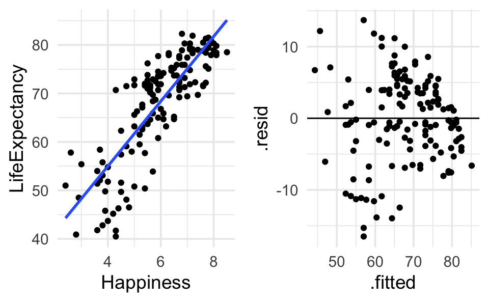

Intervals of interest: mean response, individual response, and parameter(s).

predict.lm(happy.lm, newdata=list(Happiness=c(4,7)),interval=c("conf"), level=.95)
#>    fit  lwr  upr
#> 1 55.0 53.2 56.7
#> 2 75.1 73.8 76.4
predict.lm(happy.lm, newdata=list(Happiness=c(4,7)),interval=c("pred"), level=.95)
#>    fit  lwr  upr
#> 1 55.0 42.7 67.3
#> 2 75.1 62.9 87.3

happy.lm %>% tidy(conf.int = TRUE)
#> # A tibble: 2 × 7
#>   term        estimate std.error statistic  p.value conf.low conf.high
#>   <chr>          <dbl>     <dbl>     <dbl>    <dbl>    <dbl>     <dbl>
#> 1 (Intercept)    28.2      2.28       12.4 2.76e-24    23.7      32.7 
#> 2 Happiness       6.69     0.375      17.8 5.78e-38     5.95      7.43

4.7.3.1 Residuals in R

We skipped the residuals section, so you are not responsible for finding residuals in R, but the R code is here for completion in case you are interested:

happy.lm %>% augment()
#> # A tibble: 143 × 8
#>   LifeExpectancy Happiness .fitted  .resid    .hat .sigma   .cooksd .std.resid
#>            <dbl>     <dbl>   <dbl>   <dbl>   <dbl>  <dbl>     <dbl>      <dbl>
#> 1           76.2       5.5    65.0  11.2   0.00765   6.09 0.0128        1.83  
#> 2           71.7       5.6    65.7   6.00  0.00737   6.14 0.00357       0.980 
#> 3           41.7       4.3    57.0 -15.3   0.0168    6.02 0.0539       -2.51  
#> 4           74.8       7.1    75.7  -0.944 0.0122    6.16 0.000148     -0.155 
#> 5           71.7       5      61.7  10.0   0.0101    6.10 0.0138        1.64  
#> 6           80.9       7.9    81.1  -0.198 0.0216    6.16 0.0000118    -0.0326
#> # ℹ 137 more rows

3 t-tests vs SLR

5 Analysis of Categorical Data