5 Analysis of Categorical Data

(Section 6.3 in Kuiper and Sklar (2013).)

5.1 Categorical Inference

In either an observational study or a randomized experiment, we are often interested in assessing the statistical significance of the differences we see: Is the observed difference too big to have reasonably occurred just due to chance? To answer the question, we will use

• simulation
• mathematical probability models.

Example 5.1 Back Pain & Botox, Chance and Rossman (2018), Foster et al. (2001)
The randomized clinical trial examined whether the drug botulinum toxin A (Botox) is helpful for reducing pain among patients who suffer from chronic low back pain. The 31 subjects who participated in the study were randomly assigned to one of two treatment groups: 16 received a placebo of normal saline and the other 15 received the drug itself. The subjects’ pain levels were evaluated at the beginning of the study and again after eight weeks. The researchers found that 2 of the 16 subjects who received the saline experienced a substantial reduction in pain, compared to 9 of the 15 subjects who received the actual drug.

1. Is this an experiment or an observational study?
   
2. Explain the importance of using the “placebo” treatment of saline.
   
3. Create the two-way table for summarizing the data, putting the explanatory variable as the rows and the response variable as the columns
   
4. Calculate the conditional proportions of pain reduction in the two groups. Display the results as a segmented bar graph. Comment on the preliminary analysis.

	pain reduction	no pain reduction
Botox	9	6	15
placebo	2	14	16
	11	20	31

\[\begin{eqnarray*} \mbox{risk}_{\mbox{placebo}} = \frac{2}{16} &=& 0.125\\ \mbox{risk}_{\mbox{Botox}} = \frac{9}{15} &=& 0.6\\ RR &=& 4.8 \end{eqnarray*}\]

backpain <- data.frame(treatment = c(rep("placebo", 16), rep("Botox", 15)),
                     outcome = c(rep("reduction", 2), rep("no_reduction", 14), 
                                 rep("reduction", 9), rep("no_reduction", 6)))
backpain %>%
  table()
#>          outcome
#> treatment no_reduction reduction
#>   Botox              6         9
#>   placebo           14         2

backpain %>% glimpse()
#> Rows: 31
#> Columns: 2
#> $ treatment <chr> "placebo", "placebo", "placebo", "placebo", "placebo", "plac…
#> $ outcome   <chr> "reduction", "reduction", "no_reduction", "no_reduction", "n…

Note that sometimes it makes sense for the y-axis to be count and sometimes it makes sense for the y-axis to be percent. Probably doesn’t matter much here, you should choose the bar plot that seems most informative to you.

backpain %>%
  ggplot(aes(x = treatment)) + 
  geom_bar(aes(fill = outcome), position = "fill") +
  ylab("percentage")

backpain %>%
  ggplot(aes(x = treatment)) + 
  geom_bar(aes(fill = outcome))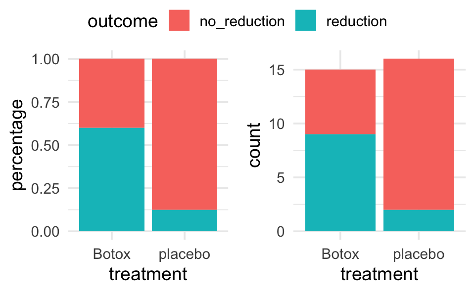

5. If there was no association between the treatment and the back pain relief, about how many of the 11 “successes” would you expect to see in each group? Did the researchers observe more successes in the saline group than expected (if the drug had no effect) or fewer successes than expected? Is this in the direction conjectured by the researchers?

6. Is is possible that the drug has absolutely no effect on back pain? That the differences were simply due to chance or random variability? How likely is that?

Simulation

• 11 red “success” cards (pain reduction); 20 black “failure” cards (no pain reduction)

• randomly deal out (i.e. shuffle) 15 cards to the treatment group and 16 cards to the placebo group.

• count how many people in the treatment group were successes? Repeat 5 times.

• process

  • what do the cards represent?
  • what does shuffling the cards represent?
  • what implicit assumption about the two groups did the shuffling of cards represent?
  • what observational units would be represented by the dots on the dotplot?
  • why would we count the number of repetitions with 9 or more “successes”?

• Repeat simulation using the two-way table applet: [http://www.rossmanchance.com/applets/2021/chisqshuffle/ChiSqShuffle.htm]

• summary

  • How many reps?
  • How many as extreme as the true data?
  • What proportion are at least as extreme as the true data?
  • Do our data support the researchers conjecture?
  • What if the actual data had been 7 successes in the treatment group (and 4 in the placebo group)?

Definition 5.1 p-value The p-value is the probability of seeing our results or more extreme if there is nothing interesting going on with the data. (This is the same definition of p-value that you will always use in this class and in your own research.)

Notice that regardless of whether or not the drug has an effect, the data will be different each time (think: new 31 people). The small p-value allows us to draw cause-and-effect conclusions, but doesn’t necessarily allow us to infer to a larger population. Why not?

low cutoff	p-value	high cutoff	evidence
	p-value \(\leq\)	0.001	very strong evidence
0.001	\(<\) p-value \(\leq\)	0.01	strong evidence
0.01	\(<\) p-value \(\leq\)	0.05	moderate evidence
0.05	\(<\) p-value \(\leq\)	0.10	weak but suggestive evidence
0.10	\(<\) p-value		little or no evidence

5.1.1 Simulation using R

The simulation from the applet can be recreated using the infer package in R. Note the different pieces of the simulation using functions like specify(), hypothesize(), generate(), and calculate(). Also notice that this particular function works best using the difference in proportions (which we discussed in class is equivalent to recording the single count of Botox patients who had reduced back pain).

Step 1. Calculate the observed difference in proportion of patients with reduced back pain. Note that as with linear regression we continue to use the syntax: response variable ~ explanatory variable.

Step 2. Go through the simulation steps, just like the applet.

• specify() the variables
  
• hypothesize() about the null claim
  
• generate() many permutations of the data
  
• calculate() the statistic of interest for all the different permutations

Step 3. Plot a histogram representing the differences in proportions for all the many permuted tables. The plot represents the distribution of the differences in proportion under the null hypothesis.

Step 4. Calculate the p-value from the sampling distribution generated in Step 3.

library(infer)

# Step 1.
diff_props <- backpain %>%
  specify(outcome ~ treatment, success = "reduction") %>%
  calculate(stat = "diff in props", order = c("Botox", "placebo")) %>%
  pull()

diff_props  # print to screen to see the observed difference
#> [1] 0.475

# Step 2.
nulldist <- backpain %>%
  specify(outcome ~ treatment, success = "reduction") %>%
  hypothesize(null = "independence") %>%
  generate(reps = 1000, type = "permute") %>%
  calculate(stat = "diff in props", order = c("Botox", "placebo"))

# Step 3.
nulldist %>%
  ggplot(aes(x = stat)) + 
  geom_histogram() + 
  geom_vline(xintercept = diff_props, col = "red")

# Step 4.
# note that the average (mean) of TRUE and FALSE is a proportion
nulldist %>%
  summarize(mean(stat >= diff_props))
#> # A tibble: 1 × 1
#>   `mean(stat >= diff_props)`
#>                        <dbl>
#> 1                      0.007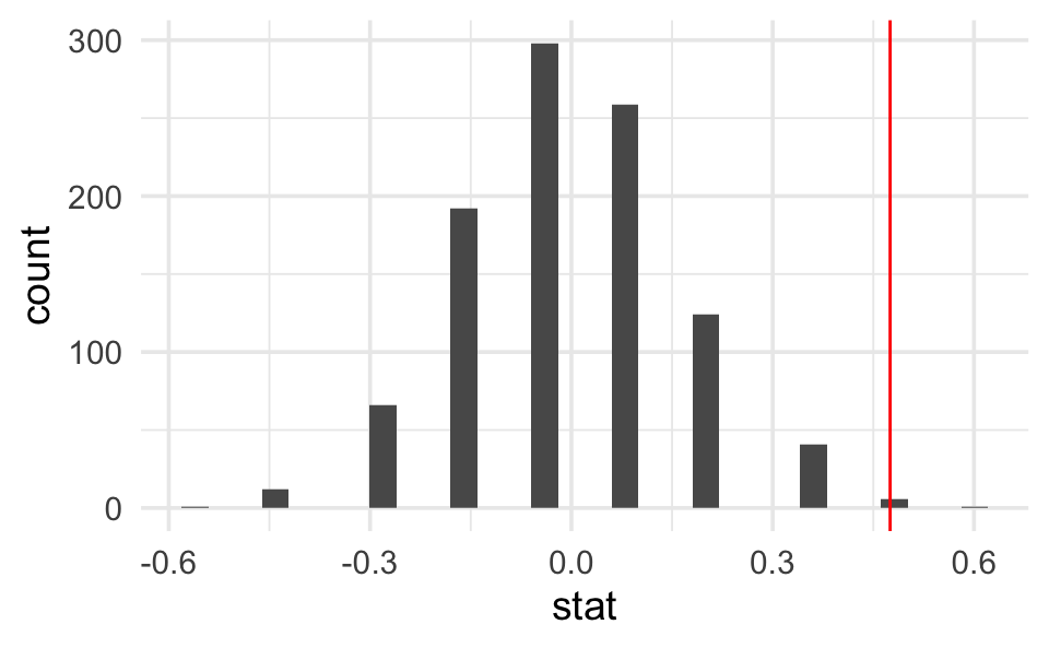

5.2 Fisher’s Exact Test

(Section 6.4 in Kuiper and Sklar (2013), great detailed explanation!)

Because we have a fixed sample, we use the hypergeometric distribution to enumerate the possible ways of choosing our data or more extreme given fixed row and column totals.

	pain reduction	no pain reduction
Botox	9 = x	6	15 = n
placebo	2	14	16
	11 = M	20 = N - M	31 = N

To make it simpler, let’s say I have 5 items (N=5), and I want to choose 3 of them (n=3). How many ways can I do that?

SSSNN, SSNSN, SSNNS, SNSSN, SNSNS, SNNSS, NSSSN, NSSNS, NSNSS, NNSSS [5!/ 3! 2!] (S = select, N = not selected)

So, how many different ways can I select 11 people (out of 31) to be my “pain reduction” group? That is the total number of different groups of size 11 from 31. But really, we want our groups to be of a certain breakdown. We need 2 (of 16) to have gotten the placebo and 9 (of 15) to have gotten the Botox treatment.

Definition 5.2 Hypergeometric Probability For any \(2 \times 2\) table when there are N observations with M total successes , the probability of observing x successes in a sample of size n is:

\[\begin{eqnarray*} P(X=x) = \frac{\# \mbox{ of ways to select x successes and n-x failures}}{\# \mbox{ of ways to select n subjects}} = \frac{ { M \choose x} {N-M \choose n-x}}{{N \choose n}}\\ \end{eqnarray*}\]

Find the P(X=2)

We can now find EXACT probabilities associated with the following hypotheses. \[\begin{eqnarray*} &&H_0: p_{pl} = p_{btx}\\ &&H_a: p_{pl} < p_{btx}\\ &&p = \mbox{true probability of no pain}\\ \end{eqnarray*}\]

Is this a one- or two-sided test? Why? [Note: the conditions here include that the row and column totals are fixed – a conditional test of independence. However, the research project in the back of chapter 6 extends the permutation test to demonstrated that the probabilities hold even under alternative technical conditions.

Note also that we get an exact probability with no conditions needed about the sample size being big enough (we can use Fisher’s Exact Test even when true probabilities are close to 0 or 1.]

5.3 Testing independence of two categorical variables

(Sections 6.5, 6.6, 6.7 in Kuiper and Sklar (2013). We are skipping Chi-square tests in Spring 2023.)

5.3.1 \(\chi^2\) tests

(Section 6.6 in Kuiper and Sklar (2013).)

2x2… but also rxc \((p_a = p_b = p_c)\)

We can also use \(\chi^2\) tests to evaluate \(r \times c\) contingency tables. Our main question now will be whether there is an association between two categorical variables of interest. Note that we are now generalizing what we did with the Botox and back pain example. Are the two variables independent? If the two variables are independent, then the state of one variable is not related to the probability of the different outcomes of the other variable.

If the data were sampled in such a way that we have random samples of both the explanatory and response variables (e.g., cross classification study), then we typically do a test of association:

\[\begin{eqnarray*} H_0: && \mbox{ the two variables are independent}\\ H_a: && \mbox{ the two variables are not independent} \end{eqnarray*}\]

If the data are sampled in such a way that the response is measured across specified populations (as in the example below), we typically do a test of homogeneity of proportions. For example,

\[\begin{eqnarray*} H_0: && p_1 = p_2 = p_3\\ H_a: && \mbox{not } H_0 \end{eqnarray*}\] where \(p=P(\mbox{success})\) for each of groups 1,2,3.

How do we get expected frequencies? The same mathematics hold regardless of the type of test (i.e., sampling mechanism used to collect the data). If, in fact,the variables are independent, then we should be able to multiply their probabilities. If the probabilities are the same, we expect the overall proportion of each response variable to be the same as the proportion of the response variable in each explanatory group. And the math in the example below follows directly.

Example 5.2 The table below show the observed distributions of ABO blood type in three random samples of African Americans living in different locations. The three datasets, collected in the 1950s by three different investigators, are reproduced in (Mourant, Kopec, and Domaniewsa-Sobczak 1976).

			Blood	Type
		A	B	AB	O	Total
Location	(Florida)	122	117	19	244	502
	(Iowa)	1781	1351	289	3301	6722
	(Missouri)	353	269	60	713	1395
	Total	2256	1737	368	4258	8619

5.3.1.1 Test of Homogeneity of Proportions (equivalent mathematically to independence)

If there is no difference in blood type proportions across the groups, then:

\[\begin{eqnarray*} P(AB | FL) = P(AB | IA) = P(AB | MO) = P(AB) \end{eqnarray*}\]

We will use \(\widehat{P}(AB) = \frac{368}{8619}\) as baseline for expectation (under \(H_0)\) for all the groups. That is, we would expect,

\[\begin{eqnarray*} \# \mbox{expected for AB blood and Iowa} &=& \frac{368}{8619} \cdot 6722\\ \end{eqnarray*}\]

5.3.1.2 Test of Independence (equivalent mathematically to homogeneity of proporitions)

\[\begin{eqnarray*} P(\mbox{ cond1 & cond2}) &=& P(\mbox{cond1}) P(\mbox{cond2}) \mbox{ if variables 1 and 2 are independent}\\ &&\\ P(AB \mbox{ blood & Iowa}) &=& P(AB \mbox{ blood}) P(\mbox{Iowa}) \\ &=& \bigg( \frac{368}{8619}\bigg) \bigg( \frac{6722}{8619} \bigg)\\ &=& 0.0333\\ &&\\ \# \mbox{expected for AB blood and Iowa} &=& 0.033 \cdot 8619\\ &=& \frac{368 \cdot 6722}{8619}\\ &&\\ E_{i,j} &=& \frac{(i \mbox{ row total})(j \mbox{ col total})}{\mbox{grand total}}\\ \end{eqnarray*}\]

And the expected values under the null hypothesis…

			Blood	Type
		A	B	AB	O	Total
Location	(Florida)	131.4	101.17	21.43	248.00	502
	(Iowa)	1759.47	1354.69	287.00	3320.83	6722
	(Missouri)	365.14	281.14	59.56	689.16	1395
	Total	2256	1737	368	4258	8619

\[\begin{eqnarray*} X^2 &=& \sum_{all cells} \frac{( O - E)^2}{E}\\ &=& 5.65\\ \mbox{p-value} &=& P(\chi^2_6 \geq 5.65) \\ &=& 1 - pchisq(5.65, 6)\\ &=& 0.464 \end{eqnarray*}\]

We cannot reject the null hypothesis. Again, we have no evidence against the null hypothesis that blood types are independently distributed in the various regions.

How do we know if our test statistic is a big number or not? Well, it turns out that the test statistic \((X^2)\) will have an approximate \(\chi^2\) distribution with degrees of freedom = \((r- 1)\cdot (c-1).\) As long as:

• We have a random sample from the population.
  
• We expect at least 1 observation in every cell \((E_i \geq 1 \forall i)\)
  
• We expect at least 5 observations in 80% of the cells \((E_i \geq 5\) for 80% of \(i)\)

When there are only two populations, the \(\chi^2\) procedure is equivalent to the two-sided z-test for proportions. The chi-squared test statistic is the square of the z-test statistic. That is, the chi-squared test is exactly the same as the two-sided alternative for the z-test.

use chi-square if you have multiple populations

use z-test if you want one-sided tests or confidence intervals.

5.4 Parameter Estimation

(Section 6.8 in Kuiper and Sklar (2013).)

Definition 5.3 Data Types Data are often classified as

• Categorical - each unit is assigned to a category
  
• Quantitative - each observational unit is assigned a numerical value
  
• (Binary - a special case of categorical with 2 categories, e.g. male/female)

Table 6.6 on page 193 of Kuiper and Sklar (2013) is excellent and worth looking at.

Example 5.3 Popcorn & Lung Disease Chance and Rossman (2018)

In May 2000, eight people who had worked at the same microwave-popcorn production plant reported to the Missouri Department of Health with fixed obstructive lung disease. These workers had become ill between 1993 and 2000 while employed at the plant. On the basis of these cases, in November 2000 researchers began conducting medical examinations and environmental surveys of workers employed at the plant to assess their occupational exposures to certain compounds (Kreiss, et al., 2002). As part of the study, current employees at the plant underwent spirometric testing. This measures FVC – forced viral capacity – the volume of air that can be maximally, forcefully exhaled. On this test, 31 employees had abnormal results, including 21 with airway obstruction. A total of 116 employees were tested.

Researchers were curious as to whether the baseline risk was high among microwave-popcorn workers. The plant itself was broken into several areas, some of which were separate from the popcorn production area. Air and dust samples in each job area were measured to determine the exposure to diacetyl, and marker of organic chemical exposure. Employees were classified into two groups: a “low-exposure group” and a “high-exposure group,” determined by how long an employee spent at different jobs within the plant and the average exposure in that job area. Of the 21 participants with airway obstruction, 6 were from the low-exposure group and 15 were from the high-exposure group. Both exposure groups contained 58 total employees.

How can we tell if popcorn production is related to lung disease? Consider High / Low exposure:

	Airway obstructed	Airway not obstructed
low exposure	6	52	58
high exposure	15	43	58
	21	95	116

Is 21 a lot of people? Can we compare 6 vs. 15? What should we look at? proportions (always a number between 0 and 1). Look at your data (graphically and numerically). Segmented bar graph (mosaic plot):

Is there a difference in the two groups? Look at the difference in proportions or risk:

\[\begin{eqnarray*} 6/58 = 0.103 & 15/58=0.2586 & \Delta = 0.156\\ p_1 = 0.65 & p_2 = 0.494 & \Delta = 0.156\\ p_1 = 0.001 & p_2 = 0.157 & \Delta = 0.156\\ \end{eqnarray*}\]

5.4.1 Differences in Proportions

It turns out that the sampling distribution of the difference in the sample proportions (of success) across two independent groups can be modeled by the normal distribution if we have reasonably large sample sizes (CLT).

To ensure the accuracy of the test, check whether np and n(1-p) is bigger than 5 in both samples is usually adequate. A more precise check is \(n_s \hat{p}_c\) and \(n_s(1-\hat{p}_c)\) are both greater than 5; \(n_s\) is the smaller of the two sample sizes and \(\hat{p}_c\)is the sample proportion when the two samples are combined into one.

Note: \[\begin{eqnarray*} \hat{p}_1 - \hat{p}_2 \sim N\Bigg(p_1 - p_2, \sqrt{\frac{p_1(1-p_1)}{n_1} + \frac{p_2(1-p_2)}{n_2}}\Bigg) \end{eqnarray*}\]

When testing independence, we assume that \(p_1=p_2,\) so we use the pooled estimate of the proportion to calculate the SE: \[\begin{eqnarray*} SE(\hat{p}_1 - \hat{p}_2) = \sqrt{ \hat{p}_c(1-\hat{p}_c) \bigg(\frac{1}{n_1} + \frac{1}{n_2}\bigg)} \end{eqnarray*}\]

So, when testing, the appropriate test statistic is: \[\begin{eqnarray*} Z = \frac{\hat{p}_1 - \hat{p}_2 - 0}{ \sqrt{ \hat{p}_c(1-\hat{p}_c) (\frac{1}{n_1} + \frac{1}{n_2})}} \end{eqnarray*}\]

5.4.1.1 Confidence interval for \(p_1 - p_2\)

We can’t pool our estimate for the SE, but everything else stays the same…

\[\begin{eqnarray*} SE(\hat{p}_1 - \hat{p}_2) = \sqrt{\frac{\hat{p}_1(1-\hat{p}_1)}{n_1} + \frac{\hat{p}_2(1-\hat{p}_2)}{n_2}} \end{eqnarray*}\]

The main idea here is to determine whether two categorical variables are independent. That is, does knowledge of the value of one variable tell me something about the probability of the other variable (gender and pregnancy). We’re going to talk about two different ways to approach this problem.

5.4.2 Relative Risk

Definition 5.4 Relative Risk The relative risk (RR) is the ratio of risks for each group. We say, “The risk of success is RR times higher for those in group 1 compared to those in group 2.”

\[\begin{eqnarray*} \mbox{relative risk} &=& \frac{\mbox{risk group 1}}{\mbox{risk group 2}}\\ &=& \frac{\mbox{proportion of successes in group 1}}{\mbox{proportion of successes in group 2}}\\ \mbox{RR} &=& \frac{p_1}{p_2} = \frac{p_1}{p_2}\\ \widehat{\mbox{RR}} &=& \frac{\hat{p}_1}{\hat{p}_2} \end{eqnarray*}\]

\(\widehat{RR}\) in the popcorn example is \(\frac{15/58}{6/58} = 2.5.\) We say, “The risk of airway obstruction is 2.5 times higher for those in high exposure group compared to those in the low exposure group.” What about

• sample size?
  
• baseline risk?

5.4.2.1 Confidence Interval for RR

Due to some theory that we won’t cover, we use the fact that:

\[SE(\ln (\widehat{RR})) \approx \sqrt{\frac{(1 - \hat{p}_1)}{n_1 \hat{p}_1} + \frac{(1-\hat{p}_2)}{n_2 \hat{p}_2}}\]

And more theory we won’t cover that tells us:

\[ \ln(\widehat{RR}) \stackrel{\mbox{approx}}{\sim} N\Bigg( \ln(RR), \sqrt{\frac{(1 - \hat{p}_1)}{n_1 \hat{p}_1} + \frac{(1-\hat{p}_2)}{n_2 \hat{p}_2}} \Bigg) \]

A \((1-\alpha)100\%\) CI for the \(\ln(RR)\) is: \[\begin{eqnarray*} \ln(\widehat{RR}) \pm z_{1-\alpha/2} SE(\ln(\widehat{RR})) \end{eqnarray*}\]

Which gives a \((1-\alpha)100\%\) CI for the \(RR\): \[\begin{eqnarray*} (e^{\ln(\widehat{RR}) - z_{1-\alpha/2} SE(\ln(\widehat{RR}))}, e^{\ln(\widehat{RR}) + z_{1-\alpha/2} SE(\ln(\widehat{RR}))}) \end{eqnarray*}\]

5.4.3 Odds Ratios

A related concept to risk is odds. It is often used in horse racing, where “success” is typically defined as losing. So, if the odds are 3 to 1 we would expect to lose 3/4 of the time.

Definition 5.5 Odds Ratio A related concept to risk is odds. It is often used in horse racing, where “success” is typically defined as losing. So, if the odds are 3 to 1 we would expect to lose 3/4 of the time. The odds ratio (OR) is the ratio of odds for each group. We say, “The odds of success is OR times higher for those in group 1 compared to those group 2.”

\(\mbox{ }\)

\[\begin{align} \mbox{odds} &= \frac{\mbox{proportion of successes}}{\mbox{proportion of failures}}\\ &= \frac{\mbox{number of successes}}{\mbox{number of failures}} = \theta\\ \widehat{\mbox{odds}} &= \hat{\theta}\\ \mbox{odds ratio} &= \frac{\mbox{odds group 1}}{\mbox{odds group 2}} \\ \mbox{OR} &= \frac{\theta_1}{\theta_2} = \frac{p_1/(1-p_1)}{p_2/(1-p_2)}= \frac{p_1/(1-p_1)}{p_2/(1-p_2)}\\ \widehat{\mbox{OR}} &= \frac{\hat{\theta}_1}{\hat{\theta}_2} = \frac{\hat{p}_1/(1-\hat{p}_1)}{\hat{p}_2/(1-\hat{p}_2)}\\ \end{align}\]

\(\widehat{OR}\) in the popcorn example is \(\frac{15/43}{6/52} = 3.02.\) We say, “The odds of airway obstruction are 3 times higher for those in the high exposure group compared to those in the low exposure group.”

OR is more extreme than RR

Without loss of generality, assume the true \(RR > 1,\) implying \(p_1 / p_2 > 1\) and \(p_1 > p_2.\)

Note the following sequence of consequences:

\[\begin{eqnarray*} RR = \frac{p_1}{p_2} &>& 1\\ \frac{1 - p_1}{1 - p_2} &<& 1\\ \frac{ 1 / (1 - p_1)}{1 / (1 - p_2)} &>& 1\\ \frac{p_1}{p_2} \cdot \frac{ 1 / (1 - p_1)}{1 / (1 - p_2)} &>& \frac{p_1}{p_2}\\ OR &>& RR \end{eqnarray*}\]

Other considerations:

• Observational study (who worked in each place?)
  
• Cross sectional (only one point in time)
  
• Healthy worker effect (who stayed home sick?)
  
• Explanatory variable is one that is a potential explanation for any changes (here exposure level).
  
• Response variable is the measured outcome of interest (here airway obstruction).

Example 5.4 Smoking & Lung Cancer Chance and Rossman (2018)

After World War II, evidence began mounting that there was a link between cigarette smoking and pulmonary carcinoma (lung cancer). In the 1950s, two now classic articles were published on the subject. One of these studies was conducted in the United States by Wynder and Graham (1950). They found records from a large number (684) of patients with proven bronchiogenic carcinoma (a specific form of lung cancer) in hospitals in California, Colorado, Missouri, New Jersey, New York, Ohio, Pennsylvania, and Utah. They personally interviewed 634 of the subjects to identify their smoking habits, occupation, exposure to dust and fumes, alcohol intake, education, and cause of death of parents and siblings. Thirty-three subjects completed mailed questionnaires, and information for the other 17 was obtained from family members or close acquaintances. Of those in the study, the researchers focused on 605 male patients with the same form of lung cancer. Another 1332 hospital patients with similar age and economic distribution (including 780 males) without lung cancer were interviewed by these researchers in St. Louis and by other researchers in Boston, Cleveland, and Hines, Illinois.

The following two-way table replicates the counts for the 605 male patients with the same form of cancer and for the “control-group” of 780 males.

		patients	controls
none	\(<\) 1/day	8	114
light	1-9/day	14	90
mod heavy	10-15/day	61	148
heavy	16-20/day	213	278
excessive	21-34/day	187	90
chain	35\(+\)/day	122	60

Given the results of the study, do you think we can generalize from the sample to the population? Explain and make it clear that you know the difference between a sample and a population.

	cancer	healthy
chain smoking	122	60	182
no smoking	8	114	122
	130	174	304

• Causation?
  
• Case-control study (605 with lung cancer, 780 without… baseline rate?)

Group A	Group B
expl = smoking status	expl = lung cancer
resp = lung cancer	resp = smoking status

• If lung cancer is considered a success and no smoking is baseline:

\[\begin{eqnarray*} \widehat{RR} &=& \frac{122/182}{8/122} = 10.22\\ \widehat{OR} &=& \frac{122/60}{8/114} = 28.9\\ \end{eqnarray*}\] The risk of lung cancer is 10.22 times higher for those who smoke than for those who don’t smoke.

The odds of lung cancer is 28.9 times higher for those who smoke than for those who don’t smoke.

• If chain smoking is considered a success and healthy is baseline:

\[\begin{eqnarray*} \widehat{RR} &=& \frac{122/130}{60/174} = 2.7\\ \widehat{OR} &=& \frac{122/8}{60/114} = 28.9\\ \end{eqnarray*}\] The risk of smoking is 2.7 times higher for those who have lung cancer than for those who don’t have lung cancer.

The odds of smoking is 28.9 times higher for those who have lung cancer than for those who don’t have lung cancer.

5.4.3.1 Important Take-Away

We want to interpret as the probability of cancer if smoker. But those individual proportions and individual odds are not estimable. Therefore the relative risk is also not estimable.

BUT because the odds ratio is invariant to which is the response variable and which is the explanatory variable, the odds ratio is estimable!

AND the interpretation for the study will be:

The odds of lung cancer is 28.9 times higher for those who smoke than for those who don’t smoke.

We know the risk of being a light smoker if you have lung cancer but we do not know the risk of lung cancer if you are a light smoker. Let’s say we have a population of 1,000,000 people:

	cancer	healthy
light smoking	49,000	51,000	100,000
no smoking	1,000	899,000	900,000
	50,000	950,000	1,000,000

\[\begin{eqnarray*} P(\mbox{light} | \mbox{lung cancer}) &=& \frac{49,000}{50,000} = 0.98\\ P(\mbox{lung cancer} | \mbox{light}) &=& \frac{49,000}{100,000} = 0.49\\ \end{eqnarray*}\]

• What is the explanatory variable?
• What is the response variable?
• relative risk?
• odds ratio?

Group A	Group B
expl = smoking status	expl = lung cancer
resp = lung cancer	resp = smoking status

• If lung cancer is considered a success and no smoking is baseline:

\[\begin{eqnarray*} RR &=& \frac{49/100}{1/900} = 441\\ OR &=& \frac{49/51}{1/899} = 863.75\\ \end{eqnarray*}\]

• If light smoking is considered a success and healthy is baseline:

\[\begin{eqnarray*} RR &=& \frac{49/50}{51/950} = 18.25\\ OR &=& \frac{49/1}{51/899} = 863.75\\ \end{eqnarray*}\]

OR is the same no matter which variable you choose as explanatory versus response! Though, in general, we still prefer to know baseline odds or baseline risk (which we can’t know with a case-control study).

Example 5.5 More on Smoking & Lung Cancer, Chance and Rossman (2018)
Now we have a cohort prospective study. (Previously we had a case-control retrospective study). Now do we have baseline risk estimates? Yes! But be careful, we can’t conclude causation, because the study is still observational.

5.4.3.2 Confidence Interval for OR

Due to some theory that we won’t cover:

\[\begin{eqnarray*} SE(\ln (\widehat{OR})) &\approx& \sqrt{\frac{1}{n_1 \hat{p}_1 (1-\hat{p}_1)} + \frac{1}{n_2 \hat{p}_2 (1-\hat{p}_2)}} \end{eqnarray*}\]

And more theory we won’t cover that tells us:

\[ \ln(\widehat{OR}) \stackrel{\mbox{approx}}{\sim} N\Bigg( \ln(OR), \sqrt{\frac{1}{n_1 \hat{p}_1 (1-\hat{p}_1)} + \frac{1}{n_2 \hat{p}_2 (1-\hat{p}_2)}} \Bigg) \]

Note that your book introduces \(SE(\ln(\widehat{OR}))\) in the context of hypothesis testing where the null, \(H_0: p_1 = p_2,\) is assumed to be true. If the null is true, you’d prefer an estimate for the proportion of success to be based on the entire sample:

\[\begin{eqnarray*} SE(\ln (\widehat{OR})) &\approx& \sqrt{\frac{1}{n_1 \hat{p} (1-\hat{p})} + \frac{1}{n_2 \hat{p}(1-\hat{p})}} \end{eqnarray*}\]

So, a \((1-\alpha)100\%\) CI for the \(\ln(OR)\) is: \[\begin{eqnarray*} \ln(\widehat{OR}) \pm z_{1-\alpha/2} SE(\ln(\widehat{OR})) \end{eqnarray*}\]

Which gives a \((1-\alpha)100\%\) CI for the \(OR\): \[\begin{eqnarray*} (e^{\ln(\widehat{OR}) - z_{1-\alpha/2} SE(\ln(\widehat{OR}))}, e^{\ln(\widehat{OR}) + z_{1-\alpha/2} SE(\ln(\widehat{OR}))}) \end{eqnarray*}\]

Back to the example… \(OR = 28.9.\) \[\begin{eqnarray*} SE(\ln(\widehat{OR})) &=& \sqrt{\frac{1}{182*0.67*(1-0.67)} + \frac{1}{122*0.0656*(1-0.0656)}}\\ &=& 0.398\\ 90\% \mbox{ CI for } \ln(OR) && \ln(28.9) \pm 1.645 \cdot 0.398\\ && 3.366 \pm 1.645 \cdot 0.398\\ && (2.71, 4.02)\\ 90\% \mbox{ CI for } OR && (e^{2.71}, e^{4.02})\\ && (15.04, 55.47)\\ \end{eqnarray*}\]

We are 90% confident that the true \(\ln(OR)\) is between 2.71 and 4.02. We are 90% confident that the true \(OR\) is between 15.04 and 55.47. That is, the true odds of getting lung cancer if you smoke are somewhere between 15.04 and 55.47 times higher than if you don’t smoke, with 90% confidence.

Note 1: we use the theory which allows us to understand the sampling distribution for the \(\ln(\widehat{OR}).\) We use the process for creating CIs to transform back to \(OR.\)

Note 2: We do not use the t-distribution here because we are not estimating the population standard deviation.

Note 3: There are not good general guidelines for checking whether the sample sizes are large enough for the normal approximation. Most authorities agree that one can get away with smaller sample sizes here than for the differences of two proportions. If the sample sizes pass the rough check discussed for \(\chi^2,\) they should be large enough to support inferences based on the approximate normality of the log of the estimated odds ratio, too. (Ramsey and Schafer 2012, 541)

For the normal approximation to hold, we need the expected counts in each cell to be at least 5. (Pagano and Gauvreau 2000, 355)

Note 4: If any of the cells are zero, many people will add 0.5 to that cell’s observed value.

Note 5: The OR will always be more extreme than the RR (one more reason to be careful…)

\[\begin{eqnarray*} \mbox{assume } && \frac{X_1 / n_1}{X_2 / n_2} = RR > 1\\ & & \\ \frac{X_1}{n_1} &=& RR \ \ \frac{X_2}{n_2}\\ \frac{X_1}{n_1 - X_1} &=& RR \ \ \bigg( \frac{n_1}{n_2} \frac{n_2 - X_2}{n_1 - X_1} \bigg) \frac{X_2}{n_2-X_2}\\ OR &=& RR \ \ \bigg(\frac{n_1}{n_2} \bigg) \frac{n_2 - X_2}{n_1 - X_1}\\ &=& RR \ \ \bigg(\frac{1/n_2}{1/n_1} \bigg) \frac{n_2 - X_2}{n_1 - X_1}\\ &=& RR \ \ \frac{1 - X_2/n_2}{1 - X_1/n_1}\\ & > & RR \end{eqnarray*}\] [\(1 - \frac{X_2}{n_2} > 1 - \frac{X_1}{n_1} \rightarrow \frac{1 - \frac{X_2}{n_2}}{1 - \frac{X_1}{n_1}} > 1\)]

Note 6: \(RR \approx OR\) if the risk is small (the denominator of the OR will be very similar to the denominator of the RR).

5.5 Types of Studies

(Section 6.9 of Kuiper and Sklar (2013).)

Definition 5.6 Explanatory variable is one that is a potential explanation for any changes in the response variable.

Definition 5.7 Response variable is the measured outcome of interest.

Definition 5.8 Case-control study: identify observational units by response

Definition 5.9 Cohort study: identify observational units by explanatory variable

Definition 5.10 Cross-classification study: identify observational units regardless of levels of the variable.

5.5.1 Retrospective versus Prospective Studies

After much research (and asking many people who do not all agree!), I finally came across a definition of retrospective that I like. Note, however, that many many books define retrospective as synonymous with case-control. That is, they define a retrospective study to be one in which the observational units were chosen based on their status of the response variable. I disagree with that definition. As you see below, retrospective studies are defined based on the when the variables were measured. I’ve also given a quote from the Kuiper text where retrospective is defined as any study where historic data are collected (I like this definition less).

Definition 5.11 A prospective study watches for outcomes, such as the development of a disease, during the study period. The explanatory variables are measured before the response variable occurs.

Definition 5.12 A retrospective study looks backwards and examines exposures to suspected risk or protection factors in relation to an outcome that is established at the start of the study. The explanatory variables are measured after the response has happened.

Studies can be classified further as either prospective or retrospective. We define a prospective study as one in which exposure and covariate measurements are made before the cases of illness occur. In a retrospective study these measurements are made after the cases have already occurred… Early writers referred to cohort studies as prospective studies and to case-control studies as retrospective studies because cohort studies usually begin with identification of the exposure status and then measure disease occurrence, whereas case-control studies usually begin by identifying cases and controls and then measure exposure status. The terms prospective and retrospective, however, are more usefully employed to describe the timing of disease occurrence with respect to exposure measurement. For example, case-control studies can be either prospective or retrospective. A prospective case-control study uses exposure measurements taken before disease, whereas a retrospective case-control study uses measurements taken after disease. (Rothman and Greenland 1998, 74)

Retrospective cohort studies also exist. In these designs past (medical) records are often used to collect data. As with prospective cohort studies, the objective is still to first establish groups based on an explanatory variable. However since these are past records the response variable can be collected at the same time. (Kuiper and Sklar 2013, chap. 6, page 24)

Understanding if a study is retrospective or prospective leads to having a sense of the biases within a study.

• The retrospective aspect may introduce selection bias and misclassification or information bias. With retrospective studies, the temporal relationship is frequently difficult to assess.

Disadvantages of Prospective Cohort Studies

• You may have to follow large numbers of subjects for a long time.
  
• They can be very expensive and time consuming.
  
• They are not good for rare diseases.
  
• They are not good for diseases with a long latency.
  
• Differential loss to follow up can introduce bias.

Disadvantages of Retrospective Cohort Studies

• As with prospective cohort studies, they are not good for very rare diseases.
• If one uses records that were not designed for the study, the available data may be of poor quality.
• There is frequently an absence of data on potential confounding factors if the data was recorded in the past.
• It may be difficult to identify an appropriate exposed cohort and an appropriate comparison group.
• Differential losses to follow up can also bias retrospective cohort studies.

Disadvantages from: http://sphweb.bumc.bu.edu/otlt/MPH-Modules/EP/EP713_CohortStudies/EP713_CohortStudies5.html

Examples of studies:

• cross-classification, prospective: NHANES
  
• cross-classification, retrospective: death records (if exposure is measured post-hoc)
  
• case-control, prospective: the investigator still enrolls based on outcome status, but the measurements for the outcome variable happened after the measurements for the explanatory variable (e.g., medical records on BMI or smoking status)
  
• case-control, retrospective: at the start of the study, all cases have already occurred and the investigator goes back to measure the exposure (explanatory) variable
  
• cohort, prospective: follows the selected participants to assess the proportion who develop the disease of interest
  
• cohort, retrospective: the exposure and outcomes have already happened (i.e., death records)

Which test?

(Section 6.1 of Kuiper and Sklar (2013).)

It turns out that the tests above (independence, homogeneity of proportions, homogeneity of odds) are typically equivalent with respect to their conclusions. However, they each have particular conditions related to what they are testing, but that we can generally use any of them for our hypotheses of interest. However, we need to be very careful about our interpretations!

(No goodness of fit, section 6.11 of Kuiper and Sklar (2013).)

5.6 R Example (categorical data): Botox and back pain

5.6.1 Entering and visualizing the data

backpain <- data.frame(treatment = c(rep("placebo", 16), rep("Botox", 15)),
                     outcome = c(rep("reduction", 2), rep("no reduction", 14), 
                                 rep("reduction", 9), rep("no reduction", 6)))
backpain %>%
  table()
#>          outcome
#> treatment no reduction reduction
#>   Botox              6         9
#>   placebo           14         2



backpain %>%
  ggplot(aes(x = treatment)) + 
  geom_bar(aes(fill = outcome))

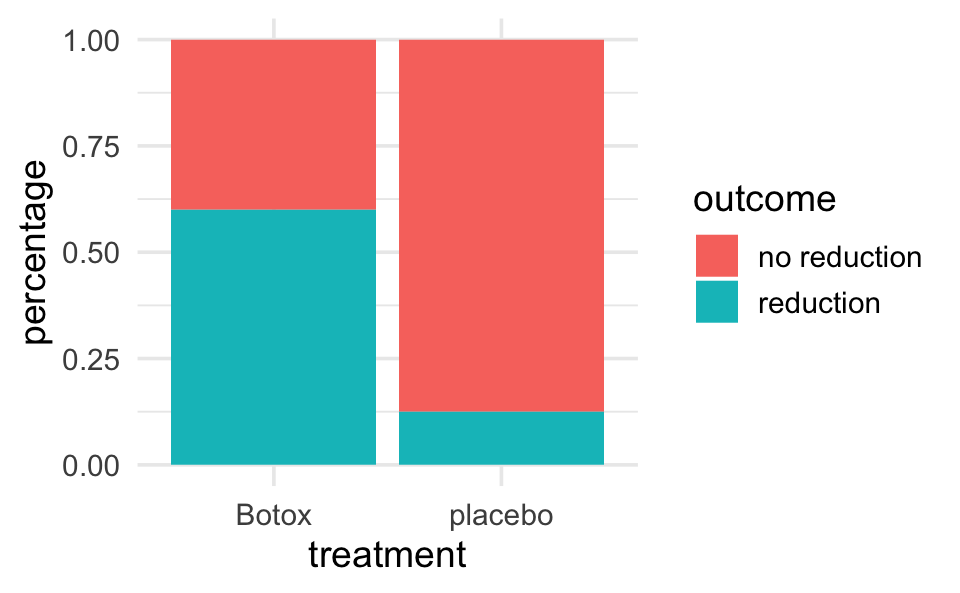
backpain %>%
  ggplot(aes(x = treatment)) + 
  geom_bar(aes(fill = outcome), position = "fill") +
  ylab("percentage")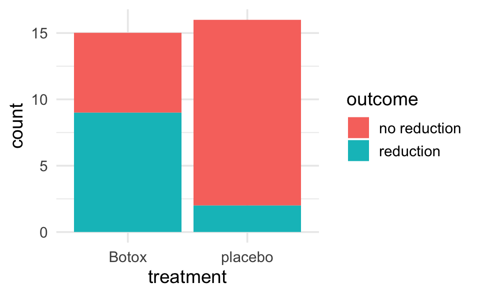

5.6.2 Simulation of Fisher’s Exact Test

library(infer)

# Step 1.
odds_ratio <- backpain %>%
  specify(outcome ~ treatment, success = "reduction") %>%
  calculate(stat = "odds ratio", order = c("Botox", "placebo")) %>%
  pull()

odds_ratio  # print to screen to see the observed difference
#> [1] 10.5

# Step 2.
nulldist <- backpain %>%
  specify(outcome ~ treatment, success = "reduction") %>%
  hypothesize(null = "independence") %>%
  generate(reps = 1000, type = "permute") %>%
  calculate(stat = "odds ratio", order = c("Botox", "placebo"))

# Step 3.
nulldist %>%
  ggplot(aes(x = stat)) + 
  geom_histogram() + 
  geom_vline(xintercept = odds_ratio, col = "red")

# Step 4.
# note that the average (mean) of TRUE and FALSE is a proportion
nulldist %>%
  summarize(mean(stat >= odds_ratio))
#> # A tibble: 1 × 1
#>   `mean(stat >= odds_ratio)`
#>                        <dbl>
#> 1                      0.016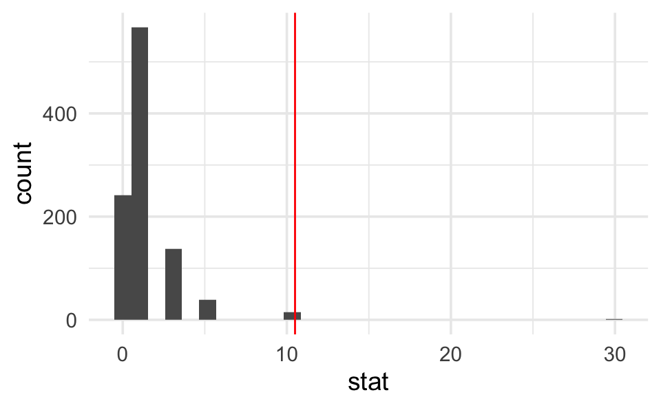

5.6.3 Fisher’s Exact Test

Note that the method used in fisher.test() to compute the CI is outside the scope of this class.

backpain %>%
  table() %>%
  fisher.test()
#> 
#>  Fisher's Exact Test for Count Data
#> 
#> data:  .
#> p-value = 0.009
#> alternative hypothesis: true odds ratio is not equal to 1
#> 95 percent confidence interval:
#>  0.00848 0.71071
#> sample estimates:
#> odds ratio 
#>      0.104

# an approximate SE for the ln(OR) is given by:
se.lnOR <- sqrt(1/(16*(2/16)*(14/16)) + 1/(15*(9/15)*(6/15)))
se.lnOR
#> [1] 0.922

5.6.4 Chi-squared Analysis

backpain %>%
  table() %>%
  chisq.test()
#> 
#>  Pearson's Chi-squared test with Yates' continuity correction
#> 
#> data:  .
#> X-squared = 6, df = 1, p-value = 0.02