15 Smoothing Methods

There are different names for the smoothing functions: smoothers, loess, lowess (locally weighted scatterplot smoothing). They are all slightly different, and we will investigate some of the nuanced differences. Note, however, the goal is to fit a model on \(X\) that predicts \(E[Y | X]\) which is not necessarily linear in \(X\). So far in the course, every model fit has been linear in the parameters (of said differently, the expected response is a linear function of the explanatory variables, which are sometimes transformed).

\[E[Y | X] = \beta_0 + \beta_1 X_1 + \beta_2 X_2 + \cdots + \beta_{p-1} X_{p-1} = f(X)\]

With ridge regression and lasso we were able to improve the model by making it simpler, but it was still linear. Linear models can only go so far, because not all relationships are linear!

We’ve talked about transformations, and relatedly, polynomial regression. That is, by including powers of the original variable (\(X\), \(X^2\), \(X^3\), etc.), the model can better fit the data.

15.1 Step functions

Step functions cut the range of a variable into K distinct regions in order to produce a qualitative variable. This has the effect of fitting a piecewise constant function.

A similar idea to to polynomial regression is to fit step functions to the data. That is, to fit a flat line for different sets of values of a given explanatory variable. Note that the flat lines don’t have any requirement that they be monotonically increasing. (Just like the polynomial fit allows for many different increasing or decreasing trends.)

Consider the following cutpoints which partition the range of \(X\): \(c_1 < c_2 < \cdots < c_K\), and create \(K+1\) new variables:

\[\begin{eqnarray*} C_0(X) &=& I(X < c_1)\\ C_1(X) &=& I(c_1 \leq X < c_2)\\ C_2(X) &=& I(c_2 \leq X < c_3)\\ &\vdots&\\ C_{K-1}(X) &=& I(c_{K-1} \leq X < c_K)\\ C_K(X) &=& I(c_K \leq X) \end{eqnarray*}\]

where \(I(\cdot)\) is the indicator function which returns a 1 if the condition is true and 0 otherwise. Note that \(C_0(X) + C_1(X) + \cdots + C_K(X) =1\), so only \(K\) predictors should be used in the model. That is:

\[E[Y_i | X_i] = \beta_0 + \beta_1 C_1(X_i) + \beta_2 C_2(X_i )+ \cdots + \beta_K C_K(X_i) \]

Note that at most one of the \(C_k\) are non-zero. \(\beta_0\) can be interpreted as the mean value of \(Y\) given that \(X < c_1\). In contrast, the mean value of\(Y\) \(c_j \leq X < c_{j+1}\) is \(\beta_0 + \beta_j\). Therefore, \(\beta_j\) is interpreted as the difference in expected response for \(X\) in \(c_j \leq X < c_{j+1}\) as compared to \(X < c_1\).

Any of the \(K\) step functions can be used to create the step function as a model on \(X\). However, it should be noted that using \(C_1, \ldots C_K\) is more intuitive than any other set of \(K\) indicator functions. Why is that? Consider the following functions and related models:

\[\begin{eqnarray*} C_0(X) &=& 1 \mbox{ if } X < 4\\ C_1(X) &=& 1 \mbox{ if } 4 <= X < 10\\ C_2(X) &=& 1 \mbox{ if } 10 <= X < 50\\ C_3(X) &=& 1 \mbox{ if } 50 <= X \end{eqnarray*}\]

Valid models can be built with any 3 of the above basis functions:

\[\begin{eqnarray*} \mbox{model1: } E[Y|X] &=& \beta_0 + \beta_1 C_1(X) + \beta_2 C_2(X) + \beta_3 C_3(X)\\ \mbox{model2: } E[Y|X] &=& \beta_0^* + \beta_1^* C_0(X) + \beta_2^* C_1(X) + \beta_3^* C_2(X) \\ \end{eqnarray*}\] n.b. The \(*\) indicates that the coefficients will differ across the two models.

Given the two different models (which lead to the exact same prediction models!), note the following:

\[\begin{eqnarray*} \mbox{model1: } E[Y| X=0] &=& \beta_0\\ \mbox{model2: } E[Y | X=0] &=& \beta_0^* + \beta_1^*\\ \mbox{model2: } E[Y | X=100] &=& \beta_0^* \end{eqnarray*}\] Which is to say, it is more intuitive to have the intercept value match with X=0. But the intercept is given when the basis functions equal zero (not necessarily when the X value equals zero).

15.1.1 Basis Functions

Polynomial and piece-wise-constant regression models are both special cases of a basis function approach to modeling. The idea is that instead of regressing on a series of different \(X\) values, you can regress on different functions of \(X\). We’ve seen this already in the form of transformations on \(X\). The basis function model is:

\[E[Y_i | X_i] = \beta_0 + \beta_1 bf_1(X_i) + \beta_2 bf_2(X_i) + \cdots + \beta_K bf_K(X_i).\]

Remember that there are no assumptions made about the explanatory variables when running the OLS model. Which is to say that functions of \(X\) cause no problem in the model as long as the variables are not collinear. Note that with polynomial regression, the basis functions are: \(bf_j(X_i) = X_i^j\). When applying step functions to the model, the basis functions are \(bf_j(X_i) = I(c_j \leq X_i < c_{j+1})\). The basis function model above can be fit using standard OLS techniques.

One of the big advantages to using OLS with basis functions is that we get to bring along all of the inference tools we covered in the first part of the course. That is, we have estimates for the standard errors of the coefficients as well as an ability to compute p-values associated with nested F-tests. The 2*SE bounds on the estimated curves are from the appropriate errors given by the predict() function on the basis function model(s).

15.2 Regression splines

Regression splines (also called smoothing splines) are more flexible than polynomials and step functions, and in fact are an extension of the two. They involve dividing the range of X into K distinct regions. Within each region, a polynomial function is fit to the data. However, these polynomials are constrained so that they join smoothly at the region boundaries, or knots. Provided that the interval is divided into enough regions, this can produce an extremely flexible fit.

By combining the ideas of polynomial fits and step functions, we can create a model which fits locally but is not required to be a horizontal line. In particular, if cubic functions are fit to each region, the model ends up as something like:

\[\begin{eqnarray} E[Y_i | X_i] = \begin{cases} \beta_{01} + \beta_{11} X_i + \beta_{21} X_i^2 + \beta_{31}X_i^3 \mbox{ if } X_i < c\\ \beta_{02} + \beta_{12} X_i + \beta_{22} X_i^2 + \beta_{32}X_i^3 \mbox{ if } X_i \geq c \end{cases} \end{eqnarray}\]

Notes:

• Any polynomial can be fit (step functions are polynomials of degree 0!)
• The fit is independent of any normality or independence assumptions. However, those assumptions are important in order to perform inference.
• If \(f(X)\) isn’t linear or polynomial in X, the model can be fit locally. Note: every function can be written as a sum of polynomials.
• Keep in mind that splines computed from truncated polynomials can be numerically unstable because the explanatory variables may be highly correlated.

Note, however, that the cubic model in the equation above has no requirement of continuity at the value \(c\). The solution is to fit a piece-wise polynomial under the constraint that the fitted curve must be continuous. Additionally, in order for the curves to seem smooth} the constraint that both the first and second derivatives are also continuous is added. Generally, for a degree-\(d\) spline: fit degree-\(d\) polynomials with continuity in derivatives up to degree \(d-1\) at each knot.

One method for fitting continuous cubic models to a partitioned \(X\) variable is to create the following function \(h(X, \xi)\) at each knot \(\xi\).

\[\begin{eqnarray*} h(X, \xi) = (X - \xi)^3_+ = \begin{cases} (X-\xi)^3 & \mbox{ if } X > \xi\\ 0 & \mbox{ otherwise} \end{cases} \end{eqnarray*}\] The following cubic spline with \(K\) knots is then modeled as \[\begin{eqnarray} E[Y_i | X_i] = \beta_0 + \beta_1 X_i + \beta_2 X_i^2 + \beta_3 X_i^3 + \beta_4 h(X_i, \xi_1) + \beta_5 h(X_i, \xi_2) + \cdots + \beta_{K+3} h(X_i, \xi_K). \end{eqnarray}\] Note that there are \(K+3\) predictors and \(K+4\) regression coefficients to model. We are using up \(K+4\) degrees of freedom.

A little bit of work can show that the spline equation will lead to continuity in the first two derivatives and discontinuity in the third derivative (with a continuous function). Proof ideas:

• for the continuity, consider only one knot. As \(X\) approaches \(\xi\) from the left, we follow the function without the \(h\) part of the function. As \(X\) approaches \(\xi\) from the right, we get arbitrarily close to the function without any \(h\).

Consider what happens for points before the second knot. That is, \(X \leq \xi_2\): \[\begin{eqnarray*} (X - \xi_1)^3 &=& X^3 - 3X^2 \xi_1 + 3X \xi_1^2 - \xi_1^3\\ E[Y | \xi_1 < X \leq \xi_2] &=& (\beta_0 - \beta_4 \xi_1^3) + (\beta_1 + \beta_4 3 \xi_1^2)X + (\beta_2 - \beta_4 3 \xi_1)X^2 + (\beta_3 + \beta_4)X^3\\ E[Y | X \leq \xi_1] &=& \beta_0 + \beta_1X + \beta_2X^2 + \beta_3 X^3\\ lim_{X \rightarrow \xi_1^-} E[Y|X] &=& \beta_0 + \beta_1 \xi_1 + \beta_2\xi_1^2 + \beta_3 \xi_1^3\\ lim_{X \rightarrow \xi_1^+} E[Y|X] &=& \beta_0 - \beta_4 \xi_1^3 + \beta_1 \xi_1 + \beta_4 3 \xi_1^3 + \beta_2\xi_1^2 - \beta_4 3 \xi_1^3 + \beta_3 \xi_1^3 + \beta_4\xi_1^3\\ &=& \beta_0 + \beta_1 \xi_1 + \beta_2\xi_1^2 + \beta_3 \xi_1^3\\ \end{eqnarray*}\]

• for the continuity in the derivatives, recall that the derivatives are with respect to \(X\). By taking the derivatives of \(E[Y_i]\) and then the limit as \(X \rightarrow \xi\), the continuity of the first few derivatives and discontinuity of later derivatives can be seen.

Knots

Knots can be placed uniformly or at places where the function is expected to change rapidly. Most often the number of knots is set and the software places them uniformly. The number of knots is directly related to the degrees of freedom of the model, so setting the degrees of freedom also sets the number of knots. Ideally, a method such as cross validation will be used to optimize the number of knots.

degrees of freedom

Note that we can fit the model based on placing the knots or based on the number of knots (specified by degrees of freedom which places df-degree internal knots). Consider the following call to our model. The number of knots will be df-degree, here, 7 knots. In the bs() function, df+1 is the number of coefficients in the model.

15.3 Local regression

Local regression is similar to splines, but differs in an important way. The regions are allowed to overlap, and indeed they do so in a very smooth way.

Local regression (loess - locally weighted scatterplot smoothing) models fit flexible, non-linear models to a point \(x_0\) using only training values that are close to \(x_0\). The distance of the training point from \(x_0\) is considered to be a weight and is given by \(K_{i0}\). We fit weighted least squares regression using the weights from the \(X\)-direction. The algorithm for local regression is given by (section 7.6, James et al. (2021)):

---

Local Regression at \(X=x_0\) (\(p=2\))

---

1. Gather the fraction \(s=k/n\) of training points whose \(X_i\) are closest to \(x_0\). \(s\) is called the span.
2. Assign a weight \(K_{i0} = K(X_i, x_0)\) to each point in the neighborhood, so that the furthest point from \(x_0\) has weight zero and the closest point has the highest weight. All but the \(k\) closest points get zero weight.
3. Fit a weighted least squares regression of the \(Y_i\) on the \(X_i\) using the \(K_{i0}\) weights. Find \(b_0\) and \(b_1\) that minimize: \[\sum_{i=1}^n K_{i0}(Y_i - b_0 - b_1 X_i)^2.\]
4. The fitted value at \(x_0\) is given by \(\hat{f}(x_0) = b_0 + b_1x_0\).
5. Repeat steps 1. - 4. for every point; the coefficients & SE are re-computed each time.

To create the smooth regression function, the points are connected by drawing a line (or surface) between each predicted value. The fraction of points with non-zero weights is given by the span, \(s=k/n\). The span plays a role similar to other tuning parameters. It can be made to produce a model similar to OLS (large span) or to produce a model which way over-fits the data (small span). Cross validation can be used to find \(s\).

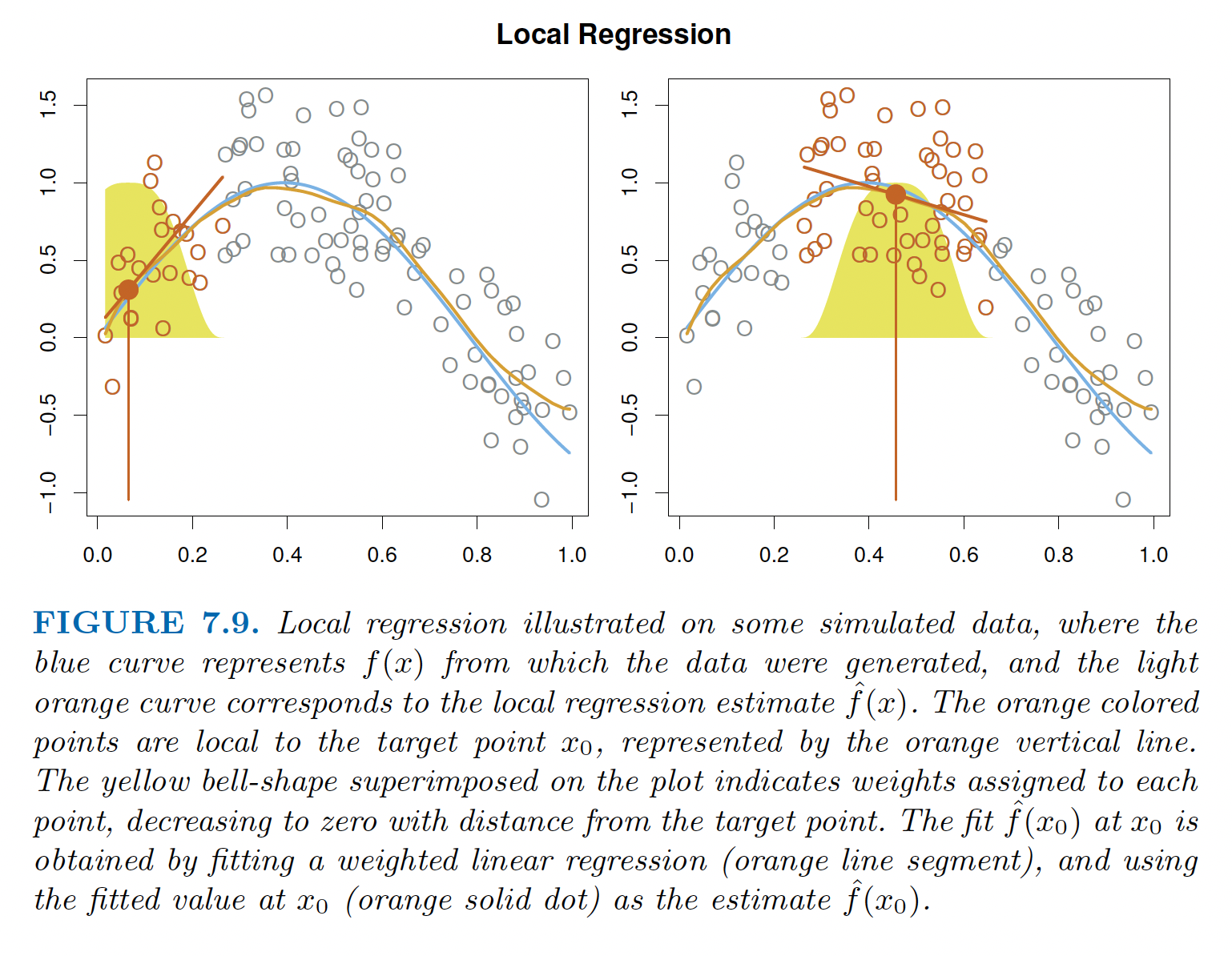
Figure 6.1: Figure 7.9 from James et al. (2021) shows weighted local regression.

Local Regression can theoretically be expanded to higher dimensions. Weighted least squares (see section 11.1 in Kutner et al. (2004)) is given by minimizing:

\[\sum_{i=1}^n w_i(Y_i - b_0 - b_1X_{i1} - \cdots - b_{p-1}X_{i,p-1})^2.\]

The normal equations are solved in the same way given coefficient estimates and standard errors as (\(W\) is the diagonal matrix of weights): \[\begin{eqnarray*} (X^t W X) b_w &=& X^t W Y\\ b_w &=& (X^t W X)^{-1} X^t W Y\\ var(b_w) &=& \sigma^2 (X^t W X)^{-1} (X^t W W X) (X^t W X)^{-1} \end{eqnarray*}\]

However, in high dimensional settings the distance to \(x_0\) might be quite large, and there will be very few points in a high dimensional neighborhood of \(x_0\). The distance problem leads to most points having zero weight (i.e., large distance) from the other points. And the regression estimates become quite variable and hard to estimate.

15.3.1 Weight function for local regression

The standard weight function used in local regression is called the tricubic weight function.

• For \(s < 1\), the neighborhood includes the proportion \(s\) of the points, and these have tricubic weighting

\[K_{i0} = \Bigg(1 - \bigg(\frac{d(x_i, x_0)}{\max_{i \in S} d(x_i, x_0)} \bigg)^3 \Bigg)^3 I\bigg[d(x_i, x_0) < \max_{i \in S} d(x_i, x_0)\bigg]\] where \(S\) defines the set of \(x_i\) values which are the \(k\) closest points to \(x_0\).

• For \(s > 1\), all points are used, with the “maximum distance” (as above) assumed to be \(s^{(1/(p-1))}\) times the actual maximum distance for \(p\) coefficients (\(p-1\) explanatory variables). \(s > 1\) means that the weights (\(K_{i0}\)) increase for larger and larger \(s\).
• Distance can be defined using any distance function, Euclidean being the default although not resistant to outliers.
• Regression is done by least squares (default) although other regression techniques can be used (e.g., Tukey’s biweight M-estimation regression… we won’t talk about that in class).
• The loess() function in R does the modeling / prediction. In ggplot2 the default method for geom_smooth() plot uses loess.

15.3.2 Imputation

Imputation is the process of replacing missing data with summary values (i.e., statistics) from the rest of the data. The biggest reason to impute data is so that the complete dataset can be used for an analysis. Notice that within the context of the models throughout the semester, it might make sense to smooth \(Y\) on some of the explanatory variables (if \(Y\) is missing for some observations), but it also might make sense to smooth \(X_1\) on the other explanatory variables (if \(X_1\) is missing and should be used in the linear model).

Keep in mind that the algorithm for creating a smooth prediction at \(x_0\) does not depend on \(x_0\) being part of the model. That is, the prediction is possible whether or not \(x_0\) has a corresponding response value.

15.3.3 Normalization

Microarrays and other high-throughput analysis techniques require normalization in order to create apples to apples comparisons. From Wikipedia, https://en.wikipedia.org/wiki/Microarray_analysis_techniques

Comparing two different arrays, or two different samples hybridized to the same array generally involves making adjustments for systematic errors introduced by differences in procedures and dye intensity effects. Dye normalization for two color arrays is often achieved by local regression. LIMMA provides a set of tools for background correction and scaling, as well as an option to average on-slide duplicate spots.[8] A common method for evaluating how well normalized an array is, is to plot an MA plot of the data.

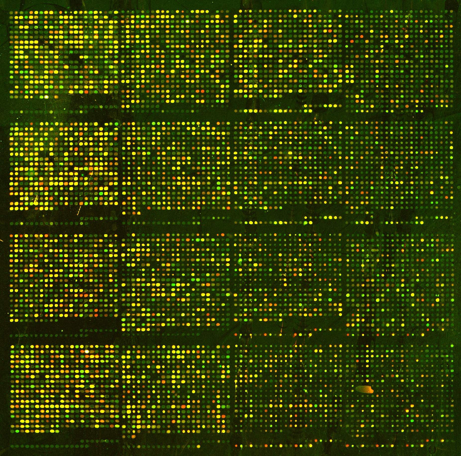
Figure 6.2: The microarray shows differing amounts of expression across two conditions (here old and young yeast). The expectation is that, on median, the dots (i.e., genes) should be yellow. As can be seen from the image, points on the left side of the microarray are dimmer than the points on the right side. The imbalance is an artifact of the technical limitations of the technique. Image due to Laura Hoopes, Pomona College.

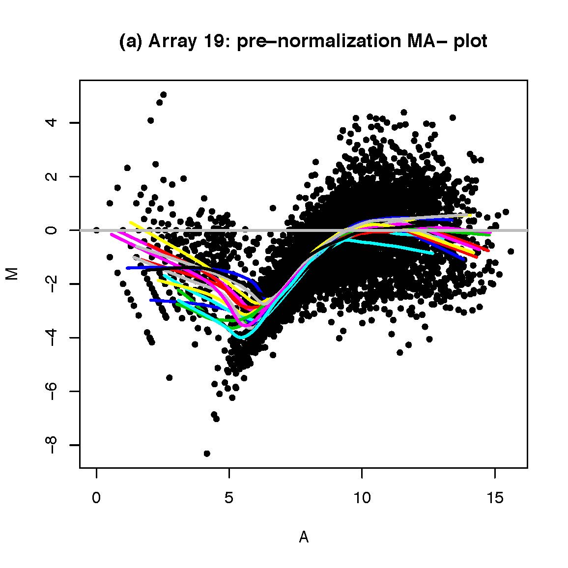
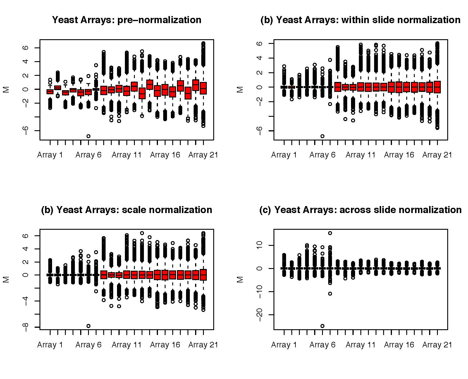
Figure 6.3: [left] M = ratio of expression, A = product of expression (total amount of expression). The different smooth curves refer to different locations on the microarray chip. To normalize, we subtract the line from each corresponding dot which can be thought of as taking the colored lines and pulling them taut. [right] By centering each array’s expression values to zero (either across the location on the chip ‘print-tip group’ or within an array itself), we can do an apples to apples comparison of the expression across different samples.

15.3.4 Prediction

After Hurricane Maria devastated Puerto Rico in September 2017, there was much discussion on how to count the resulting number of deaths. Rolando Acosta and Rafael Irizzary use loess models to predict excess deaths in Post-Hurricane Vital Statistics Expose Fragility of Puerto Rico’s Health System.

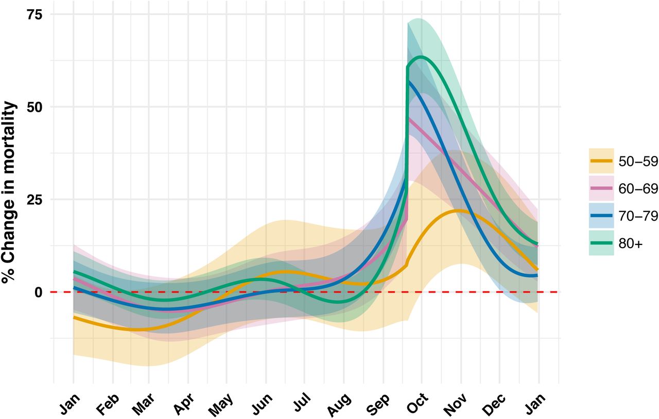
Figure 1.5: Increase in death rate as a function of date. Note the y-axis which is observed rate minus expected rate (found by using a trend line given by loess broken down by age group).

15.4 Last Thoughts…

15.4.1 Why smooth?

Advantages of smoothing

• Smoothing methods do not require a known functional relationship between \(X\) and \(Y\).
  • Regression splines do provide a functional model
  • loess does not provide a functional model
• The relationships are easy to fit
• and they retain many of the advantages of weighted least squares (including confidence estimates for the predicted values).

Disadvantages of smoothing

• Local regression can be computationally intensive, with methods giving unstable estimates in high dimensions (and at the outer range of X) due to sparsity of points.
• Regression splines have arbitrary knots which may not fit the model well.
• Although interpolation can be used to get predictions (with standard errors), there is no functional form for the relationship between \(X\) and \(Y\) with loess. Inference on coefficients is meaningless.

15.5 Inference

Keep in mind that in order to have a p-value (which is a probability), there must be a probability model. OLS assumes normal errors, and if basis functions or weighted OLS are applied using standard linear model techniques, then there should be some notion that there is an iid normal error structure. Confidence intervals also require a probability model in order to apply the standard inferential interpretations.

In particular, the wind temperature observations are not independent. There is a strong dependency between the temperature on any two consecutive days. The data are much better described by an autoregressive model if the goal is inference. (Autoregression is used, e.g., when the x-variable is time and the observations are correlated. The y-variable could be stock price or temperature. We haven’t talked about these types of models in any formal way.) If the goal is more descriptive (or simply predictive for reasons such as normalization or extrapolation), then SE values and CI bounds are not needed, and a smooth curve will probably be effective even if the technical conditions do not hold.

Don’t Forget

There is no substitute for thinking carefully about how you are modeling relationships. Whether it be linear, non-linear, sparse, locally weighted, or optimized. There will almost never be a single model which is the one right model. Instead, your expertise and practice will provide you with strategies to help come up with a model that describes your data well.

For more on kernel smoothers, see the appendix of Sheather (2009) and chapter 6 of T. Hastie, Tibshirani, and Friedman (2001).

15.6 Reflection Questions

1. How are the different types of flexible models represented in linear model form? (Step functions, polynomials, regression splines, local regression)
2. How are inferential methods applied to the models above? What are the necessary technical assumptions to make inferential claims?
3. What is a basis function? How is it used similarly / differently in step functions, polynomials, and regression splines?
4. In regression splines, how does the number of knots play a role? How do the different choice for the number of knots change the resulting model? Why would you choose to fit a model that had more or fewer knots?
5. For local regression, how do the weights play a role? What different choices could be made with respect to the weight functions?
6. For local regression, how does the span play a role? How do the different choices for the span change the resulting model? Why would you choose to fit a model that had more or fewer knots?
7. If inference claims are not accessible, what else can smoothing techniques be used for?

15.7 Ethics Considerations

The information presented here comes from a March 2022 blog by Peter Ellis on free range statistics called Smoothing charts of Supreme Court Justice nomination results. But I’ll back up a minute to provide some context.

538 politics blog

538 did a story describing how it is harder than ever to confirm a supreme court justice.

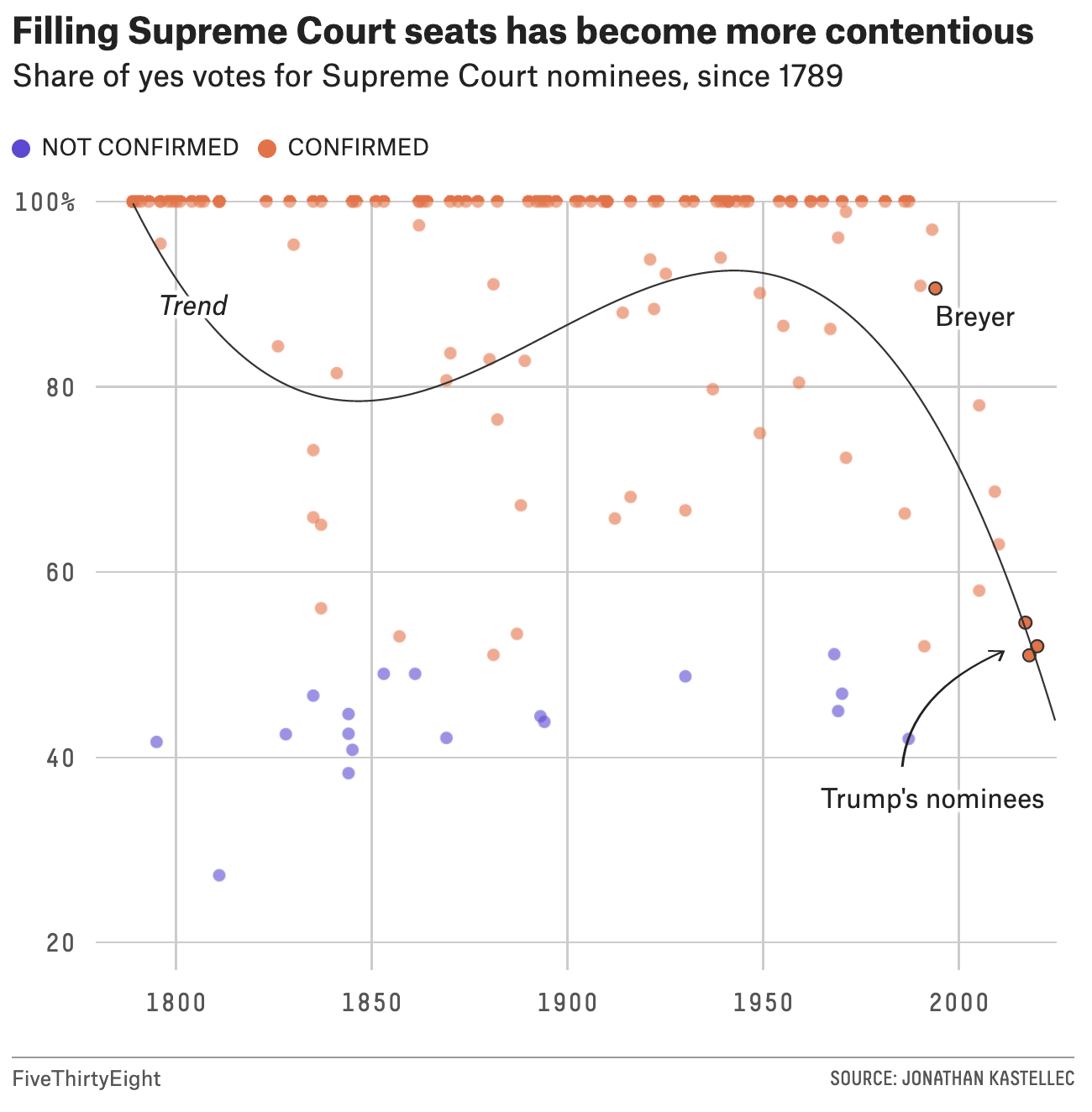
Figure 1.6: Image credit: https://fivethirtyeight.com/features/its-harder-than-ever-to-confirm-a-supreme-court-justice/

Modeling

As we know from a semester together, there are many ways to model an x-y relationship.

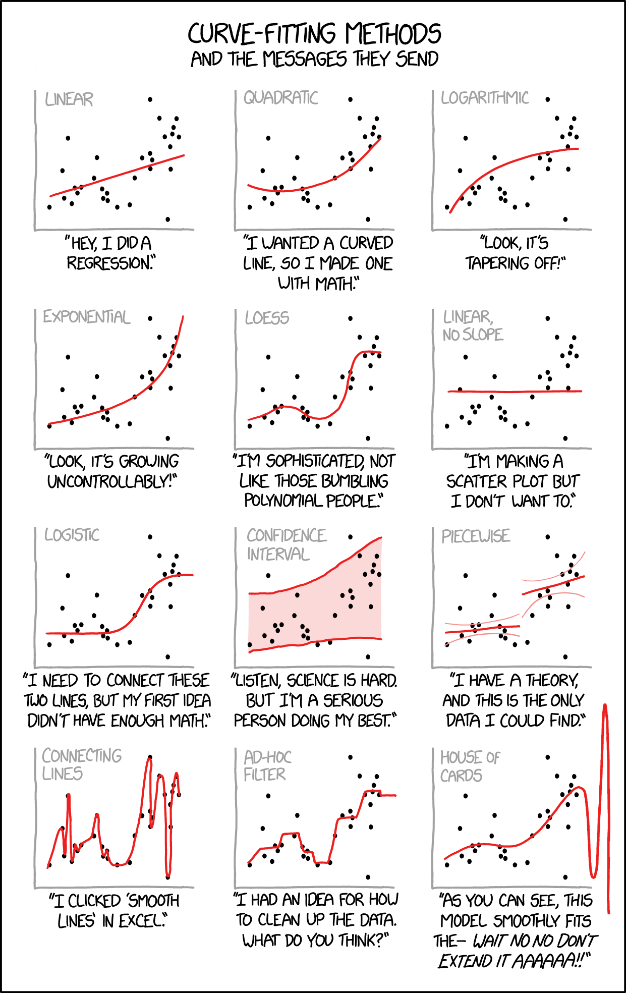
Figure 1.7: Image credit: https://xkcd.com/2048/

Twitter

People on twitter get worked up about things. The gist of their complaints is that we shouldn’t be modeling future votes based on historical trends.

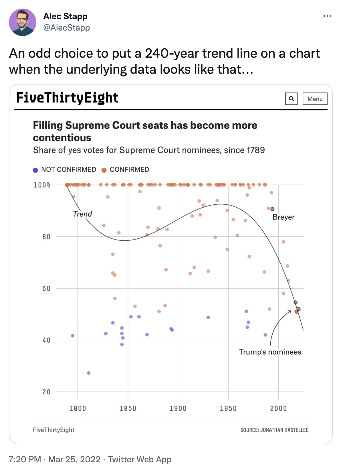
Figure 15.1: Image credit: https://twitter.com/AlecStapp/status/1507542987563323393

Five Thirty Eight said that “Supreme Court confirmations are increasingly likely to resemble party-line votes.” Is that a prediction or not?

Figure 6.4: Image credit:https://twitter.com/FiveThirtyEight/status/1488874422337482755

15.7.1 Averages

Twitter misses the point that 538 is not predicting anything. Well, at least the model doesn’t predict anything. Instead, they are using a loess smooth as an average over time. It is a descriptive model which does not try to make any inferential claims.

Ellis gives a fantastic discussion including trying different models and providing all of his R code.

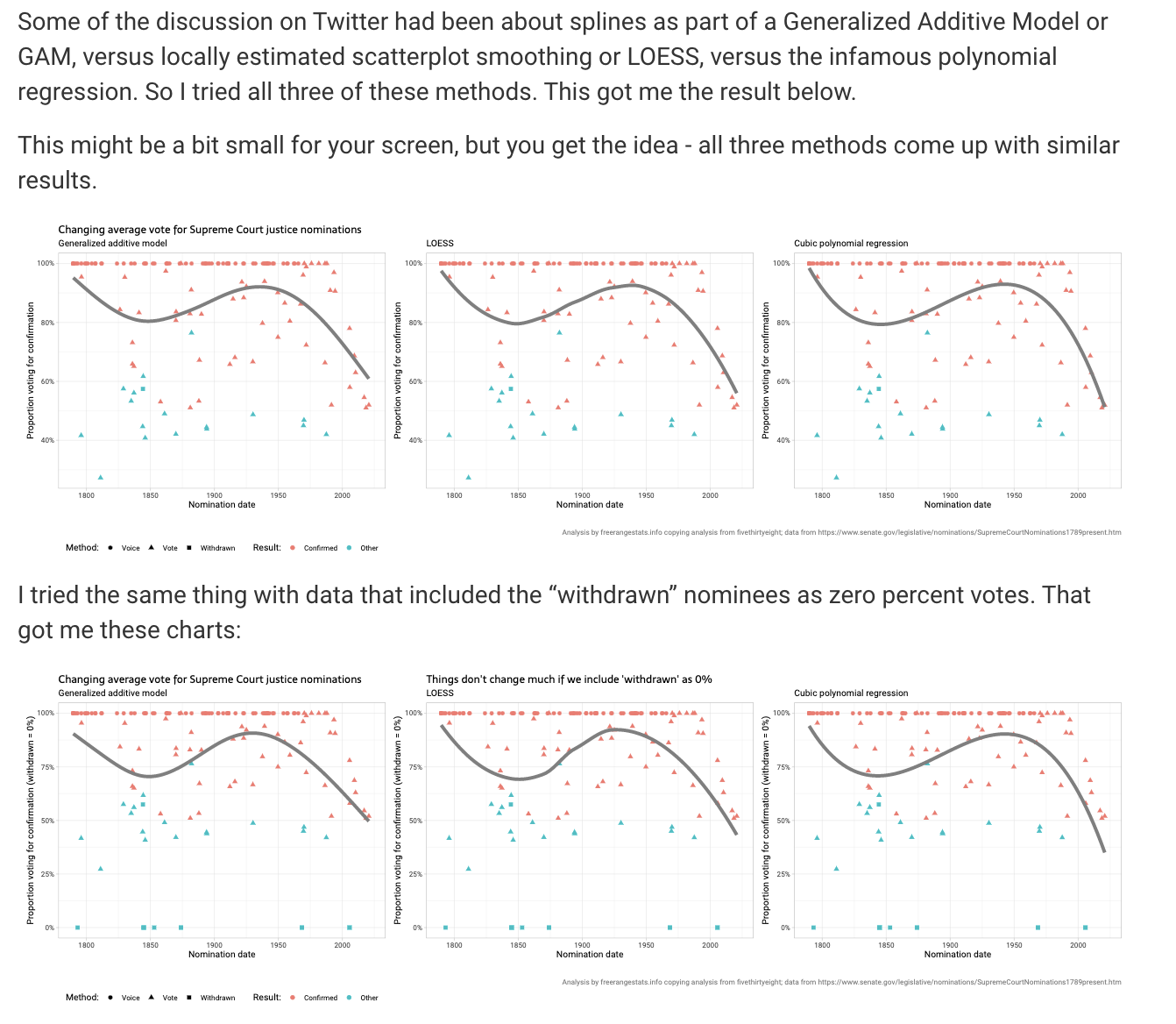
Figure 15.2: Image credit: http://freerangestats.info/blog/2022/03/26/supreme-court-nominations

15.8 R: Smoothing – NOAA

First we scrape some weather data from NOAA. The resulting data we will use is wind temperature at noon across the day of the year (for 2014) measured by a buoy off the coast of Santa Monica.

buoy_url <- "http://www.ndbc.noaa.gov/view_text_file.php?filename=46025h2014.txt.gz&dir=data/historical/stdmet/"
buoy_data_orig <- read_table(buoy_url, skip=2, col_names=FALSE)
temp <- read_table(buoy_url, n_max=1, col_names=FALSE)
temp <- unlist(strsplit(unlist(temp), "\\s+"))
names(buoy_data_orig) <- temp

buoy_data <- buoy_data_orig %>% 
  mutate(WVHT = ifelse(WVHT==99, NA, WVHT)) %>%
  mutate(DPD = ifelse(DPD==99, NA, DPD)) %>%
  mutate(APD = ifelse(APD==99, NA, APD)) %>%
  mutate(MWD = ifelse(MWD==999, NA, MWD)) %>%
  mutate(PRES = ifelse(PRES==9999, NA, PRES)) %>%
  mutate(DEWP = ifelse(DEWP==99, NA, DEWP)) %>%
  select(-VIS, -TIDE) %>% filter(`#YY`==2014)  %>% filter(hh=="12") %>%
  mutate(yearday = yday(mdy(paste(MM,DD,`#YY`, sep="-"))))

15.8.1 Polynomial Regression and Step Functions

Cubic Model

# cubic model
wind_cub <- lm(WTMP ~ poly(yearday,3, raw = TRUE), data=buoy_data)
wind_cub %>%
  tidy()

## # A tibble: 4 × 5
##   term                             estimate    std.error statistic   p.value
##   <chr>                               <dbl>        <dbl>     <dbl>     <dbl>
## 1 (Intercept)                   16.2        0.196             82.3 6.55e-229
## 2 poly(yearday, 3, raw = TRUE)1 -0.0544     0.00470          -11.6 2.16e- 26
## 3 poly(yearday, 3, raw = TRUE)2  0.000655   0.0000299         21.9 3.17e- 67
## 4 poly(yearday, 3, raw = TRUE)3 -0.00000140 0.0000000539     -26.0 2.14e- 83

# cubic predictions
wind_cub %>% 
  augment(se_fit = TRUE) %>% 
  bind_cols(buoy_data) %>%
  rename(WTMP = WTMP...1) %>%
  mutate(upper = .fitted + 2*.se.fit,
         lower = .fitted - 2*.se.fit) %>%
  ggplot(aes(x = yearday, y = WTMP)) + 
  geom_point() + 
  geom_line(aes(y = .fitted), color = "blue") + 
  geom_line(aes(y = upper), lty = 3, color = "blue") + 
  geom_line(aes(y = lower), lty = 3, color = "blue") + 
  ggtitle("Cubic Fit")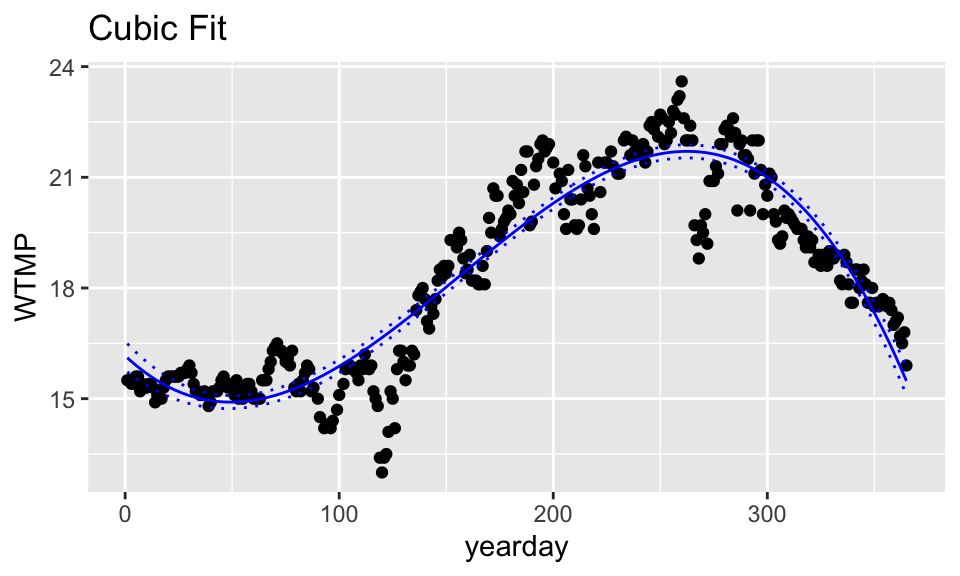

Step Functions

# cutting the yearday variable
buoy_data %>%
  summarize(cut(yearday, 4)) %>% table()

## .
## (0.636,92]   (92,183]  (183,274]  (274,365] 
##         90         86         83         90

lm(WTMP ~ cut(yearday, 4), data=buoy_data) %>%
  tidy()

## # A tibble: 4 × 5
##   term                     estimate std.error statistic   p.value
##   <chr>                       <dbl>     <dbl>     <dbl>     <dbl>
## 1 (Intercept)                 15.4      0.153    101.   1.29e-258
## 2 cut(yearday, 4)(92,183]      1.79     0.218      8.18 5.32e- 15
## 3 cut(yearday, 4)(183,274]     5.83     0.220     26.5  4.86e- 85
## 4 cut(yearday, 4)(274,365]     3.95     0.216     18.3  1.12e- 52

# step function model
wind_step <- lm(WTMP ~ cut(yearday, 4), data=buoy_data)
wind_step %>%
  tidy()

## # A tibble: 4 × 5
##   term                     estimate std.error statistic   p.value
##   <chr>                       <dbl>     <dbl>     <dbl>     <dbl>
## 1 (Intercept)                 15.4      0.153    101.   1.29e-258
## 2 cut(yearday, 4)(92,183]      1.79     0.218      8.18 5.32e- 15
## 3 cut(yearday, 4)(183,274]     5.83     0.220     26.5  4.86e- 85
## 4 cut(yearday, 4)(274,365]     3.95     0.216     18.3  1.12e- 52

#cubic predictions
wind_step %>% 
  augment(se_fit = TRUE) %>% 
  bind_cols(buoy_data) %>%
  rename(WTMP = WTMP...1) %>%
  mutate(upper = .fitted + 2*.se.fit,
         lower = .fitted - 2*.se.fit) %>%
  ggplot(aes(x = yearday, y = WTMP)) + 
  geom_point() + 
  geom_line(aes(y = .fitted), color = "blue") + 
  geom_line(aes(y = upper), lty = 3, color = "blue") + 
  geom_line(aes(y = lower), lty = 3, color = "blue") + 
  ggtitle("Step Function Fit")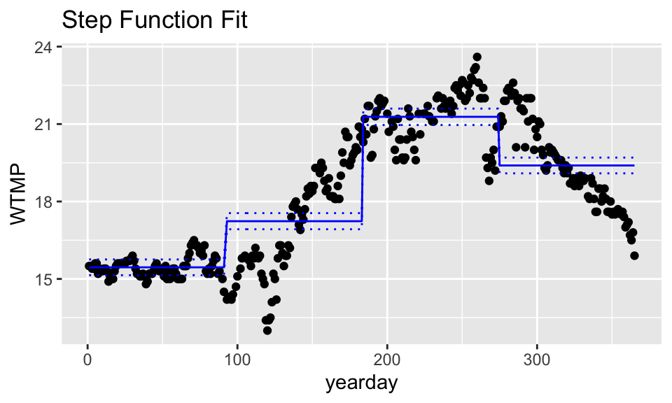

15.8.2 Regression Spline

Note that the function bs() calculates “B-Spline Basis for Polynomial Splines.” You can learn more by ?bs in the splines package. The knots argument gives “the internal breakpoints that define the spline.” The degree is the degree of the polynomial. Here, there are three internal knots.

require(splines)
year_knot1 <- bs(buoy_data$yearday, knots=c(92,183,274), degree=3)

wind_rs1 <- lm(WTMP ~ year_knot1, data=buoy_data)
wind_rs1 %>% tidy

## # A tibble: 7 × 5
##   term        estimate std.error statistic   p.value
##   <chr>          <dbl>     <dbl>     <dbl>     <dbl>
## 1 (Intercept)    14.9      0.261     56.9  1.70e-176
## 2 year_knot11     1.98     0.488      4.06 6.21e-  5
## 3 year_knot12    -2.47     0.321     -7.68 1.69e- 13
## 4 year_knot13     6.44     0.391     16.5  2.59e- 45
## 5 year_knot14     7.91     0.359     22.0  1.37e- 67
## 6 year_knot15     3.64     0.406      8.97 2.05e- 17
## 7 year_knot16     1.82     0.363      5.02 8.37e-  7

# regression spline predictions
wind_rs1 %>% 
  augment(se_fit = TRUE) %>% 
  bind_cols(buoy_data) %>%
  rename(WTMP = WTMP...1) %>%
  mutate(upper = .fitted + 2*.se.fit,
         lower = .fitted - 2*.se.fit) %>%
  ggplot(aes(x = yearday, y = WTMP)) + 
  geom_point() + 
  geom_line(aes(y = .fitted), color = "blue") + 
  geom_line(aes(y = upper), lty = 3, color = "blue") + 
  geom_line(aes(y = lower), lty = 3, color = "blue") + 
  ggtitle("Regression Spline Fit")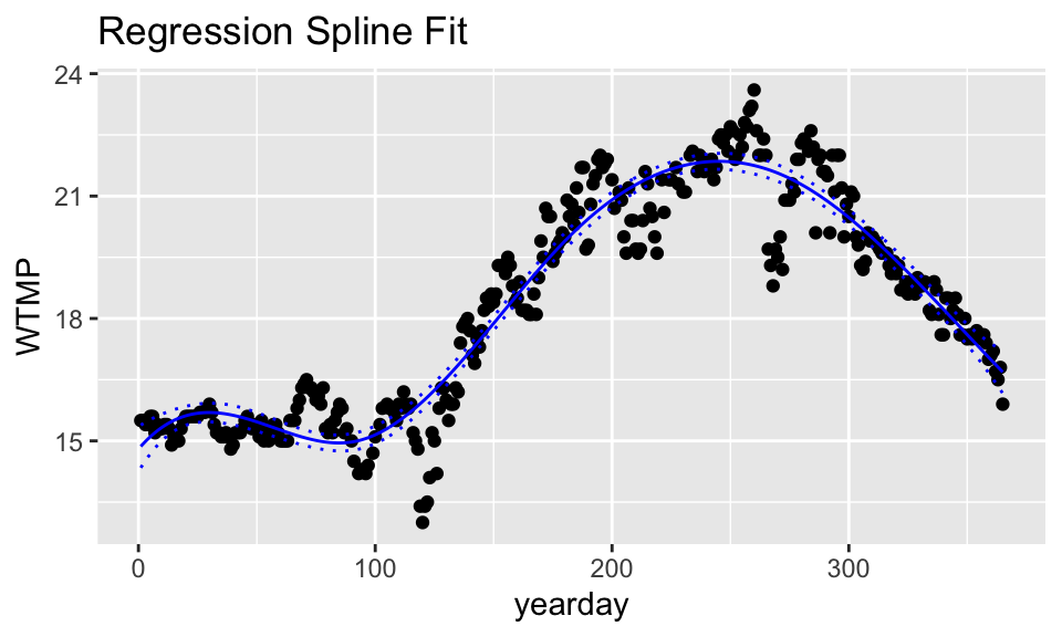

degrees of freedom

Note that we can fit the model based on placing the knots or based on the number of knots (specified by degrees of freedom which places df-degree internal knots). Consider the following call to our model. The number of knots will be df-degree, here, 7 knots. In the bs() function, df+1 is the number of coefficients in the model. The knots argument supersedes the df argument in the function.

year_knot2 <- bs(buoy_data$yearday, df=10, degree=3)
wind_rs2 <- lm(WTMP ~ year_knot2, data=buoy_data)

# note that the coefficients are very similar
wind_rs1 %>% tidy()

## # A tibble: 7 × 5
##   term        estimate std.error statistic   p.value
##   <chr>          <dbl>     <dbl>     <dbl>     <dbl>
## 1 (Intercept)    14.9      0.261     56.9  1.70e-176
## 2 year_knot11     1.98     0.488      4.06 6.21e-  5
## 3 year_knot12    -2.47     0.321     -7.68 1.69e- 13
## 4 year_knot13     6.44     0.391     16.5  2.59e- 45
## 5 year_knot14     7.91     0.359     22.0  1.37e- 67
## 6 year_knot15     3.64     0.406      8.97 2.05e- 17
## 7 year_knot16     1.82     0.363      5.02 8.37e-  7

wind_rs2 %>% tidy()

## # A tibble: 11 × 5
##    term         estimate std.error statistic   p.value
##    <chr>           <dbl>     <dbl>     <dbl>     <dbl>
##  1 (Intercept)    15.6       0.348    44.9   1.66e-144
##  2 year_knot21    -0.692     0.642    -1.08  2.82e-  1
##  3 year_knot22     0.445     0.413     1.08  2.81e-  1
##  4 year_knot23    -0.865     0.502    -1.72  8.59e-  2
##  5 year_knot24     0.207     0.412     0.501 6.17e-  1
##  6 year_knot25     6.04      0.444    13.6   6.14e- 34
##  7 year_knot26     5.21      0.439    11.9   2.22e- 27
##  8 year_knot27     7.12      0.450    15.8   1.38e- 42
##  9 year_knot28     2.98      0.496     6.01  4.73e-  9
## 10 year_knot29     2.48      0.521     4.77  2.81e-  6
## 11 year_knot210    0.914     0.489     1.87  6.26e-  2

Choosing df with CV

Below is code for using CV to determine the optimal number of knots (as a function of df) as well as the polynomial degree.

set.seed(4747)
wind_rec <- recipe(WTMP ~ yearday, data = buoy_data) %>%
  step_bs(yearday, deg_free = tune(), degree = tune())

wind_cv <- vfold_cv(buoy_data, v = 5)

wind_lm <- linear_reg() %>%
  set_engine("lm")

wind_df <- grid_regular(deg_free(range = c(5, 15)), 
                        degree(range = c(1,5)) , levels = 5)

wind_tuned <- wind_lm %>%
  tune_grid(wind_rec,
            resamples = wind_cv,
            grid = wind_df)

collect_metrics(wind_tuned)

## # A tibble: 50 × 8
##    deg_free degree .metric .estimator  mean     n std_err .config              
##       <int>  <dbl> <chr>   <chr>      <dbl> <int>   <dbl> <chr>                
##  1        5      1 rmse    standard   0.874     5 0.0337  Preprocessor01_Model1
##  2        5      1 rsq     standard   0.887     5 0.00967 Preprocessor01_Model1
##  3        7      1 rmse    standard   0.771     5 0.0227  Preprocessor02_Model1
##  4        7      1 rsq     standard   0.913     5 0.00666 Preprocessor02_Model1
##  5       10      1 rmse    standard   0.711     5 0.0244  Preprocessor03_Model1
##  6       10      1 rsq     standard   0.925     5 0.00643 Preprocessor03_Model1
##  7       12      1 rmse    standard   0.722     5 0.0286  Preprocessor04_Model1
##  8       12      1 rsq     standard   0.922     5 0.00766 Preprocessor04_Model1
##  9       15      1 rmse    standard   0.683     5 0.0441  Preprocessor05_Model1
## 10       15      1 rsq     standard   0.930     5 0.00965 Preprocessor05_Model1
## # … with 40 more rows

collect_metrics(wind_tuned) %>%
  ggplot(aes(x = deg_free, y = mean, color = as.factor(degree))) + 
  geom_line() + 
  facet_grid(.metric ~ .) + 
  labs(color = "degree") + 
  ylab("") + 
  xlab("degrees of freedom (# coefficients)")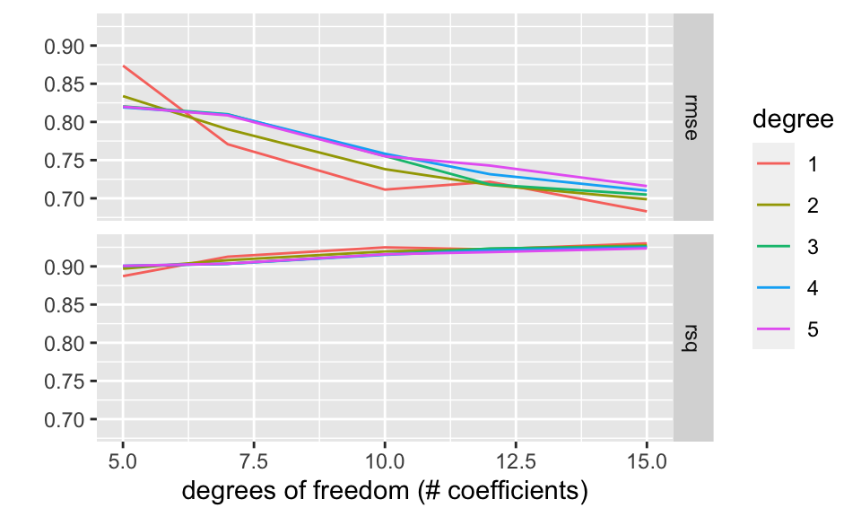

For fun, we’ve plotted two of the combinations of df and degree. If degree is 1, then the model is piece-wise linear (with 4 knots, so 5 regions). If the degree is 2, the model is piece-wise quadratic. With df = 15 there are 15 non-intercept coefficients. That means linear plus quadratic terms (=2) plus 13 knot terms (giving 14 different quadratic models across 14 different regions).

# df = 5, degree = 1
year_knot3 <- bs(buoy_data$yearday, df = 5, degree=1)

wind_rs3 <- lm(WTMP ~ year_knot3, data=buoy_data)
wind_rs3 %>% tidy

## # A tibble: 6 × 5
##   term        estimate std.error statistic   p.value
##   <chr>          <dbl>     <dbl>     <dbl>     <dbl>
## 1 (Intercept)   15.6       0.198     79.0  4.28e-222
## 2 year_knot31   -0.685     0.286     -2.40 1.71e-  2
## 3 year_knot32    1.81      0.230      7.87 4.62e- 14
## 4 year_knot33    6.37      0.250     25.5  2.95e- 81
## 5 year_knot34    5.54      0.243     22.8  1.03e- 70
## 6 year_knot35    0.959     0.279      3.44 6.61e-  4

# regression spline predictions
wind_rs3 %>% 
  augment(se_fit = TRUE) %>% 
  bind_cols(buoy_data) %>%
  rename(WTMP = WTMP...1) %>%
  mutate(upper = .fitted + 2*.se.fit,
         lower = .fitted - 2*.se.fit) %>%
  ggplot(aes(x = yearday, y = WTMP)) + 
  geom_point() + 
  geom_line(aes(y = .fitted), color = "blue") + 
  geom_line(aes(y = upper), lty = 3, color = "blue") + 
  geom_line(aes(y = lower), lty = 3, color = "blue") + 
  ggtitle("Regression Spline Fit (df = 5, degree = 1)")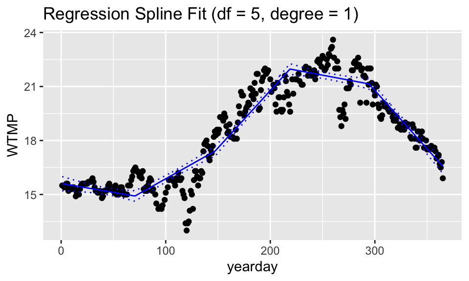

# df = 15, degree = 2
year_knot4 <- bs(buoy_data$yearday, df = 15, degree=2)

wind_rs4 <- lm(WTMP ~ year_knot4, data=buoy_data)
wind_rs4 %>% tidy

## # A tibble: 16 × 5
##    term         estimate std.error statistic   p.value
##    <chr>           <dbl>     <dbl>     <dbl>     <dbl>
##  1 (Intercept)    15.3       0.328    46.7   3.84e-148
##  2 year_knot41     0.308     0.551     0.559 5.77e-  1
##  3 year_knot42    -0.191     0.362    -0.529 5.97e-  1
##  4 year_knot43     0.314     0.416     0.756 4.50e-  1
##  5 year_knot44     0.364     0.403     0.904 3.67e-  1
##  6 year_knot45    -1.08      0.399    -2.70  7.34e-  3
##  7 year_knot46     3.01      0.397     7.59  3.15e- 13
##  8 year_knot47     3.87      0.398     9.72  8.20e- 20
##  9 year_knot48     6.25      0.400    15.6   1.43e- 41
## 10 year_knot49     4.94      0.412    12.0   8.52e- 28
## 11 year_knot410    7.58      0.395    19.2   9.34e- 56
## 12 year_knot411    5.51      0.399    13.8   1.23e- 34
## 13 year_knot412    5.86      0.401    14.6   9.66e- 38
## 14 year_knot413    2.89      0.411     7.03  1.14e- 11
## 15 year_knot414    2.86      0.451     6.35  7.26e- 10
## 16 year_knot415    1.03      0.463     2.22  2.71e-  2

# regression spline predictions
wind_rs4 %>% 
  augment(se_fit = TRUE) %>% 
  bind_cols(buoy_data) %>%
  rename(WTMP = WTMP...1) %>%
  mutate(upper = .fitted + 2*.se.fit,
         lower = .fitted - 2*.se.fit) %>%
  ggplot(aes(x = yearday, y = WTMP)) + 
  geom_point() + 
  geom_line(aes(y = .fitted), color = "blue") + 
  geom_line(aes(y = upper), lty = 3, color = "blue") + 
  geom_line(aes(y = lower), lty = 3, color = "blue") + 
  ggtitle("Regression Spline Fit (df = 15, degree = 2)")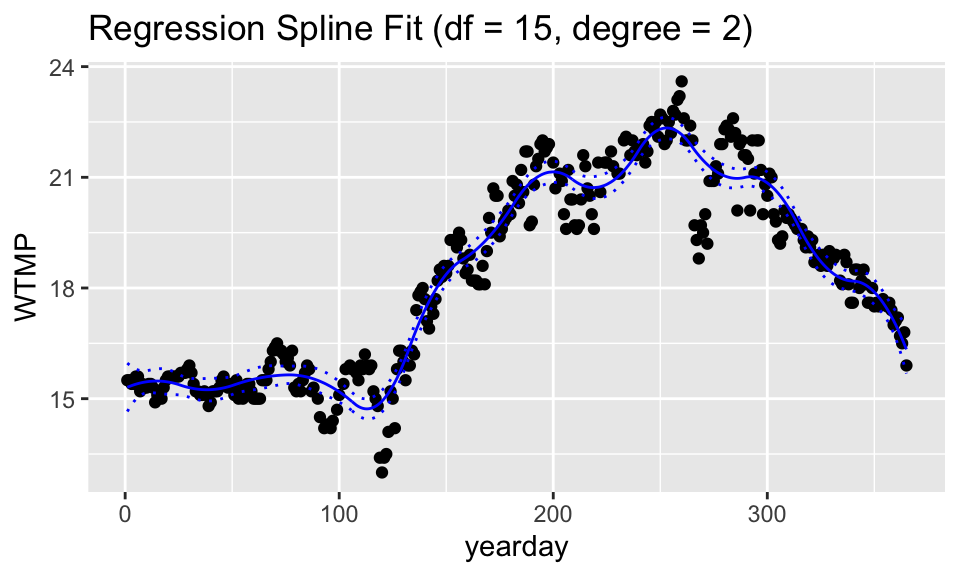

15.8.3 Local Regression (loess)

wind_lo <- loess(WTMP ~ yearday, span=.3, data=buoy_data)

# loess predictions
wind_lo %>% 
  augment(se_fit = TRUE) %>% 
  bind_cols(buoy_data) %>%
  rename(WTMP = WTMP...1, yearday = yearday...2) %>%
  mutate(upper = .fitted + 2*.se.fit,
         lower = .fitted - 2*.se.fit) %>%
  ggplot(aes(x = yearday, y = WTMP)) + 
  geom_point() + 
  geom_line(aes(y = .fitted), color = "blue") + 
  geom_line(aes(y = upper), lty = 3, color = "blue") + 
  geom_line(aes(y = lower), lty = 3, color = "blue") + 
  ggtitle("Loess Fit")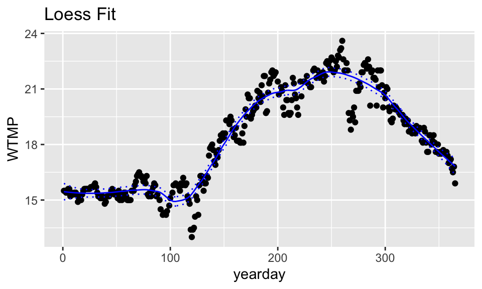

Choosing the span with CV (or not)

Like with regression splines, cross validation can be used to set the span for loess. Unfortunately, there is not an easy tidymodels way to cross validate to find the span (although the logic for doing so is the same).

Instead, in the plots below, a loess model is fit for a series of different span values. Notice, however, that for the NOAA observations, the span doesn’t change the fit very much. That is because the large dataset covers the changes in the response variable. That is, the signal is quite strong.

One interesting aspect of loess() is that it does not support extrapolation, so we cannot predict for the smallest and largest points in the dataset if they are left out.

span_vals <- seq(0.05, 1, .1)
wind_full <- data.frame()

for(i in 1:length(span_vals)){
  
wind_lo <- loess(WTMP ~ yearday, 
                     span = span_vals[i],
                     data = buoy_data)

wind_lo_output <- wind_lo %>% 
  augment(se_fit = TRUE) %>% 
  bind_cols(buoy_data) %>%
  rename(WTMP = WTMP...1, yearday = yearday...2) %>%
  mutate(upper = .fitted + 2*.se.fit,
         lower = .fitted - 2*.se.fit) %>%
  mutate(span = span_vals[i]) %>%
  dplyr::select(WTMP, yearday, .fitted, upper, lower, span)

# each time we go through the loop and change the span
# the new predictions get concatenated onto the full dataset
wind_full <- wind_full %>% bind_rows(wind_lo_output)

}

wind_full %>%
  ggplot(aes(x = yearday, y = WTMP)) + 
  geom_point(alpha = .1) + 
  geom_line(aes(y = .fitted), color = "blue") + 
  geom_line(aes(y = upper), lty = 3, color = "blue") + 
  geom_line(aes(y = lower), lty = 3, color = "blue") + 
  facet_wrap(~span) + 
  ggtitle("Loess Fit (changing span)")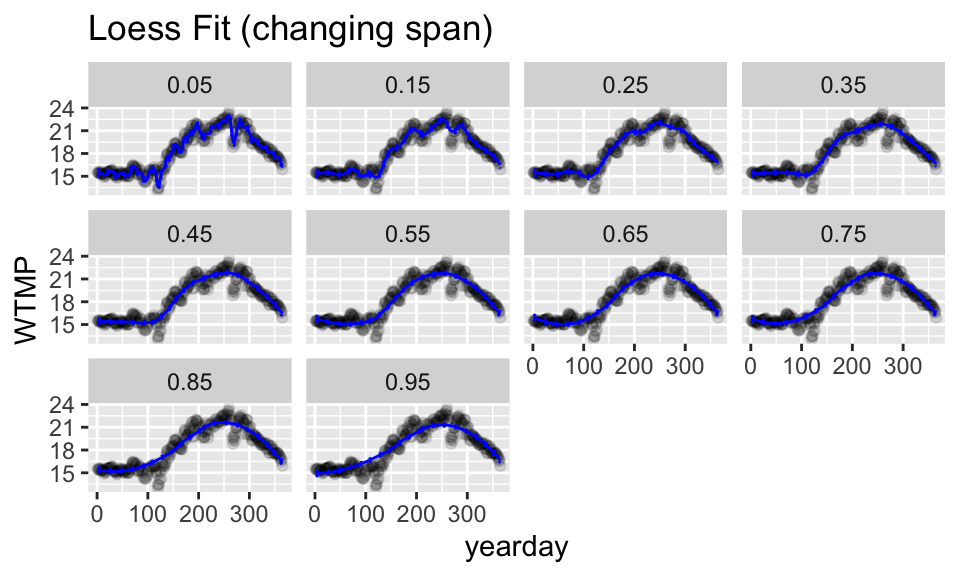

Imputing using Local Regression (loess)

The following TechNote¹⁹ shows examples of loess (local polynomial regression fitting) smoothing for various “span” values. The online R documentation (?loess) says the default span value is 0.75, but doesn’t give much guidance, nor visual examples, of how the span value affects smoothing. In addition to simply smoothing a curve, the R loess() function can be used to impute missing data points. An example of data imputation with loess() is shown.

Let’s take a sine curve, add some “noise” to it, and then see how the loess “span” parameter affects the look of the smoothed curve.

1. Create a sine curve and add some noise:

set.seed(47)
period <- 120
x <- 1:120
y <- sin(2*pi*x/period) + runif(length(x),-1,1)

sine_unif_data <- data.frame(x = x, y = y)

2. Plot the points on this noisy sine curve:

sine_unif_data %>%
  ggplot(aes(x = x, y = y)) + 
  geom_point() + 
  ggtitle("Sine Curve + Uniform Noise")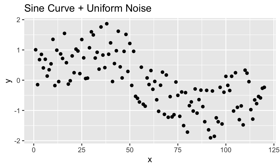

3. Apply loess smoothing using the default span value of 0.75.

y_loess <- loess(y ~ x, span=0.2, data = sine_unif_data)

4. Compute loess smoothed values for all points along the curve using `augment().

y_loess %>% augment()

## # A tibble: 120 × 4
##         y     x .fitted  .resid
##     <dbl> <int>   <dbl>   <dbl>
##  1  1.01      1   0.558  0.448 
##  2 -0.148     2   0.550 -0.697 
##  3  0.679     3   0.543  0.136 
##  4  0.853     4   0.540  0.312 
##  5  0.406     5   0.542 -0.136 
##  6  0.692     6   0.547  0.144 
##  7  0.136     7   0.554 -0.417 
##  8  0.345     8   0.560 -0.215 
##  9  0.541     9   0.571 -0.0303
## 10  1.35     10   0.589  0.761 
## # … with 110 more rows

5. Plot the loess smoothed curve along with the points that were already plotted:

y_loess %>% augment() %>%
  mutate(truth = sin(2*pi*x/period)) %>%
  ggplot(aes(x = x, y = y)) + 
  geom_point() + 
  geom_line(aes(x = x, y = .fitted)) + 
  geom_line(aes(x = x, y = truth), color = "purple") +
  ggtitle("Sine Curve + Uniform Noise")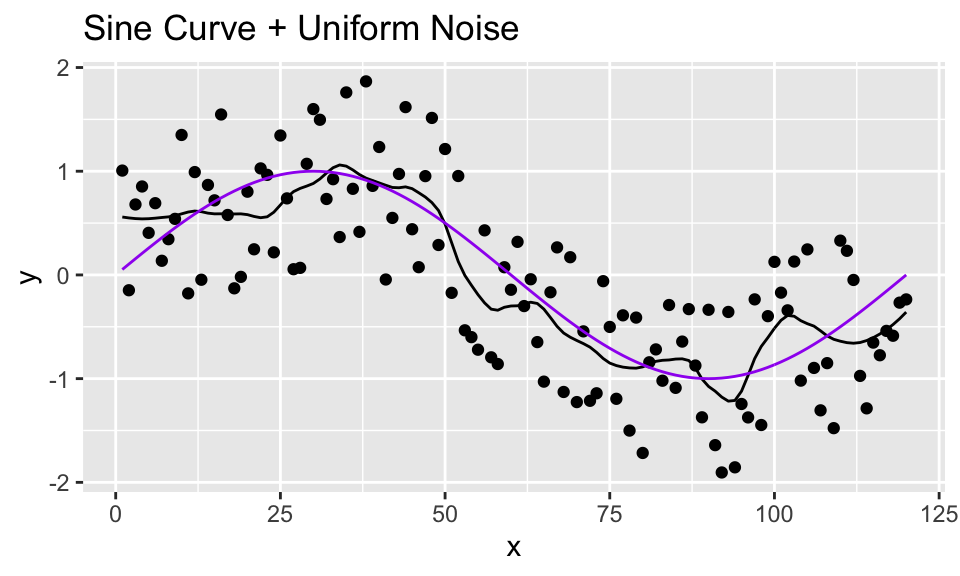

6. Repeat steps 1-5 above for various span values.

loess_unif <- data.frame()
spanlist <- c(0.10, 0.25, 0.50, 0.75, 1.00, 2.00)
for (i in 1:length(spanlist))
{
  loess_unif_pred <- loess(y ~ x, span = spanlist[i], 
                           data = sine_unif_data) %>%
    augment() %>%
    mutate(span = spanlist[i])
  
  loess_unif <- loess_unif %>% bind_rows(loess_unif_pred)
  
}
    loess_unif %>%
      mutate(truth = sin(2*pi*x/period)) %>%
      ggplot(aes(x = x, y = y)) + 
      geom_point() + 
      geom_line(aes(x = x, y = .fitted, color = as.factor(span))) + 
      geom_line(aes(x = x, y = truth), color = "black") +
      labs(color = "span") + 
      ggtitle("Sine Curve + Uniform Noise")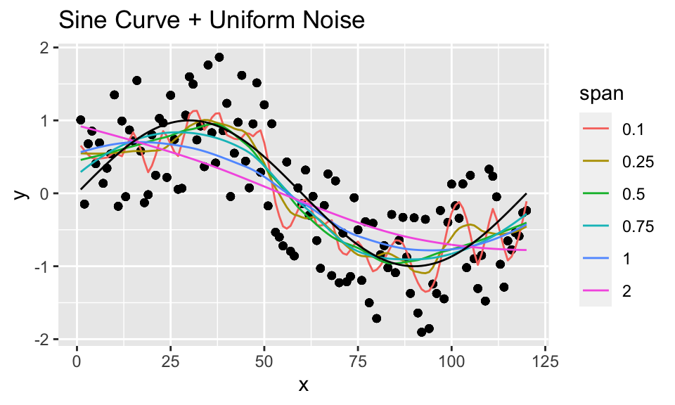

7. Compare “noise” from a uniform distribution from -1 to 1 (above) to Gaussian noise, with mean 0 and standard deviation 1.0 (below).

set.seed(47)
period <- 120
x <- 1:120
y <- sin(2*pi*x/period) + rnorm(length(x), 0, 1)

sine_norm_data <- data.frame(x = x, y = y)

loess_unif <- data.frame()
spanlist <- c(0.10, 0.25, 0.50, 0.75, 1.00, 2.00)
for (i in 1:length(spanlist))
{
  loess_unif_pred <- loess(y ~ x, span = spanlist[i], 
                           data = sine_norm_data) %>%
    augment() %>%
    mutate(span = spanlist[i])
  
  loess_unif <- loess_unif %>% bind_rows(loess_unif_pred)
  
}
    loess_unif %>%
      mutate(truth = sin(2*pi*x/period)) %>%
      ggplot(aes(x = x, y = y)) + 
      geom_point() + 
      geom_line(aes(x = x, y = .fitted, color = as.factor(span))) + 
      geom_line(aes(x = x, y = truth), color = "black") +
      labs(color = "span") + 
      ggtitle("Sine Curve + Normal Noise")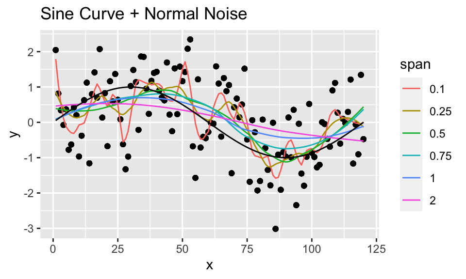

8. Let’s use loess() to impute data points. Start by taking a sine curve with noise, like computed above, but leave out 15 of the 120 data points using R’s “sample” function. Note the gaps in the (true) sine function superimposed on the points.

set.seed(47)
period <- 120
missing_pts <- sample(1:period, 15)
missing_pts

##  [1]  27  57 114  15  84   1  26  13  23  70   9  54   6  12 104

 # Create sine curve with noise
x <- 1:period
y <- sin(2*pi*x/period) + runif(length(x),-1,1) 
sine_miss_data <- data.frame(x = x, y = y) %>%
  slice(-missing_pts)


sine_miss_data %>%
  mutate(truth = sin(2*pi*x/period)) %>% 
  bind_rows(data.frame(x = missing_pts, y = NA)) %>%
  ggplot(aes(x = x, y = y)) + 
  geom_line(aes(y = truth, group = 1), color = "purple") + 
  geom_point() + 
  ggtitle("Missing data gone from model")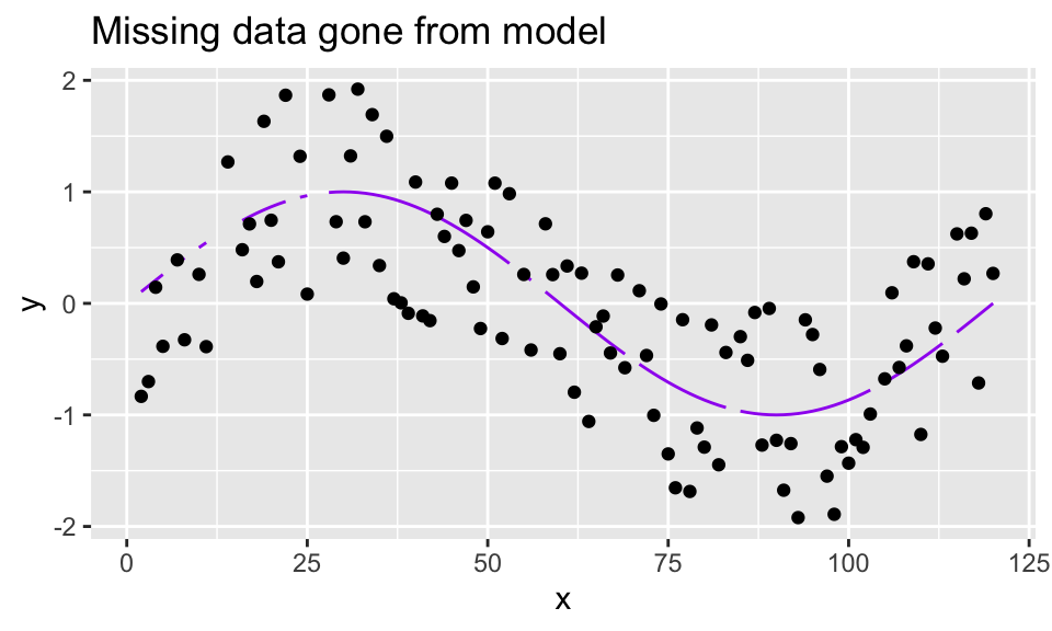

9. As before, use the loess() and augment() functions to get smoothed values at the defined points:

y_miss_loess <- loess(y ~ x, span=0.75, data = sine_miss_data)

y_miss_pred <- y_miss_loess %>% 
  augment(newdata = data.frame(x = missing_pts))

10. Use the loess and predict functions to also impute the values at the missing points:

sine_miss_data %>%
  mutate(truth = sin(2*pi*x/period)) %>% 
  bind_rows(data.frame(x = missing_pts, y = NA)) %>%
  ggplot(aes(x = x, y = y)) + 
  geom_line(aes(y = truth, group = 1), color = "purple") + 
  geom_point() +
  geom_point(data = y_miss_pred, aes(x = x, y = .fitted),
             color = "purple", size = 4) +
  ggtitle("Missing data imputed")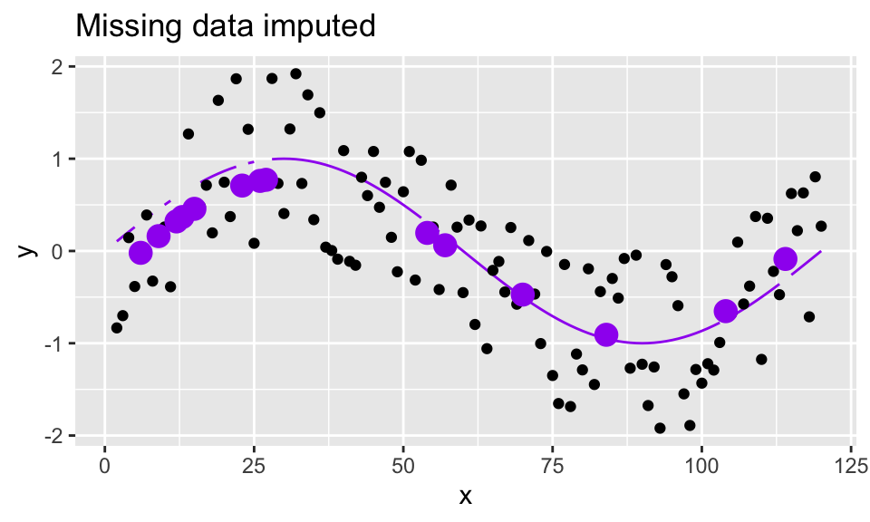

11. Compare the loess smoothed fit and imputed points for various span values.

y_miss_loess_75 <- loess(y ~ x, span=0.75, data = sine_miss_data)
y_miss_pred_75 <- y_miss_loess_75 %>% 
  augment(newdata = data.frame(x = missing_pts))

y_miss_loess_50 <- loess(y ~ x, span=0.5, data = sine_miss_data)
y_miss_pred_50 <- y_miss_loess_50 %>% 
  augment(newdata = data.frame(x = missing_pts))

y_miss_loess_1 <- loess(y ~ x, span = 1, data = sine_miss_data)
y_miss_pred_1 <- y_miss_loess_1 %>% 
  augment(newdata = data.frame(x = missing_pts))

sine_miss_data %>%
  mutate(truth = sin(2*pi*x/period)) %>% 
  bind_rows(data.frame(x = missing_pts, y = NA)) %>%
  ggplot(aes(x = x, y = y)) + 
  geom_line(aes(y = truth, group = 1), color = "black") + 
  geom_point() +
  geom_point(data = y_miss_pred_75, aes(x = x, y = .fitted),
             color = "purple", size = 4) +
  geom_point(data = y_miss_pred_50, aes(x = x, y = .fitted),
             color = "green", size = 4) +
  geom_point(data = y_miss_pred_1, aes(x = x, y = .fitted),
             color = "red", size = 4) +
  geom_line(data = y_miss_loess_75 %>% augment(), 
            aes(x = x, y = .fitted),
             color = "purple", linetype = 2) +
  geom_line(data = y_miss_loess_50 %>% augment(), 
            aes(x = x, y = .fitted),
             color = "green", linetype = 2) +
  geom_line(data = y_miss_loess_1 %>% augment(), 
            aes(x = x, y = .fitted),
             color = "red", linetype = 2) +  
  labs(title = "Missing data imputed",
       subtitle = "purple: 0.75; green = 0.5; red = 1.0")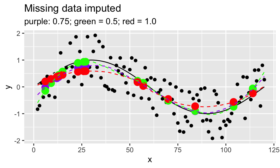

#### Discussion/Conclusion {-}

Given the sine data, span values as small as 0.10 do not provide much smoothing and can result in a “jerky” curve. Span values as large as 2.0 provide perhaps too much smoothing, at least in the cases shown above. Overall, the default value of 0.75 worked fairly well in “finding” the sine curve.