SHOW INDEXES FROM planes;| Table | Non_unique | Key_name | Seq_in_index | Column_name | Collation | Cardinality | Sub_part | Packed | Null | Index_type | Comment | Index_comment |
|---|---|---|---|---|---|---|---|---|---|---|---|---|
| planes | 0 | PRIMARY | 1 | tailnum | A | 3322 | BTREE |
The examples below use the airlines database, including the flights, carriers, airports, and planes tables.
It is worth pointing out a few aspects to loading data into SQL: keys, indexes, and partitioning.
Before we get to the definitions, consider this analogy:
Each library (
database) has books (tables). Each book (table) has pages (rows). Each page (row) has a unique page number to identify it (keyvalue); to find a particular page, you sort through the page numbers (keyvalues). But it isn’t immediately obvious where the particular page of interest is, you might have to page through the book a little bit to find the page of interest. It would be easier if you had several bookmarks throughout the book to anchor some of the page numbers. For example, if you want page 1047 and you have a bookmark on page 1050, you only have to turn back three pages. The bookmark is anindex, it helps you find the desired rows much more quickly.1
Keys are unique identifiers for each row, used primarily for connecting tables. Keys are generally not helpful for efficiency, but they are important for data integrity and relationships between tables. A key is a pointer that identifies a record. In practice, a key is one or more columns that are earmarked to uniquely identify a record in a table. Keys serve two main purposes:
PRIMARY KEY is a column or set of columns that uniquely identify each row. Primary keys cannot be NULL. Each table must always have one (and only one) PK. The PK can be made up of one column, but if that isn’t enough to uniquely identify the row, more columns may be added. Sometimes it is easier to designate a numeric column (e.g., row number) to be the PK.FOREIGN KEY is a column or set of columns that reference a primary key in a different table. The FK links two tables together, and the link is called a relationship.(There are other keys such as: Super Key, Minimal Super Key, Candidate Key, Unique Key, Alternate Key, Composite Key, Natural Key, Surrogate Key.)
Indexes are the crux of why SQL is so much more efficient than, say, R. An index is a lookup table that helps SQL keep track of which records contain certain values. By indexing the rows, SQL is able to optimize sorting and joining tables. The index is created in advance (when the table is created) and saved to disk, which can take up substantial space on the disk. Sometimes more than one variable is used to index the table. There are trade-offs to having a lot of indexes (disk space but fast wrangling) versus a few indexes (slow wrangling but less space).
A table may have more than one index but you shouldn’t add indexes to every column in a table, as these have to be updated for every addition/update/delete to the column. Rather, indexes should be added to columns that are frequently included in queries.
Indexes may not make much difference for small databases, but, as tables grow in size, queries benefit more from indexes.
In MySQL the commands SHOW KEYS and SHOW INDEXES provide information about the keys and indexes for each table (the two operations are synonymous in MySQL). Neither operation is available in DuckDB.
Notice that the planes table has a single PRIMARY key. That primary key is used to index the table. The flights table has no PRIMARY key, but it does have six different indexes: Year, Date, Origin, Dest, Carrier, and tailNum.
SHOW INDEXES FROM planes;| Table | Non_unique | Key_name | Seq_in_index | Column_name | Collation | Cardinality | Sub_part | Packed | Null | Index_type | Comment | Index_comment |
|---|---|---|---|---|---|---|---|---|---|---|---|---|
| planes | 0 | PRIMARY | 1 | tailnum | A | 3322 | BTREE |
SHOW INDEXES FROM flights;| Table | Non_unique | Key_name | Seq_in_index | Column_name | Collation | Cardinality | Sub_part | Packed | Null | Index_type | Comment | Index_comment |
|---|---|---|---|---|---|---|---|---|---|---|---|---|
| flights | 1 | Year | 1 | year | A | 7 | YES | BTREE | ||||
| flights | 1 | Date | 1 | year | A | 7 | YES | BTREE | ||||
| flights | 1 | Date | 2 | month | A | 89 | YES | BTREE | ||||
| flights | 1 | Date | 3 | day | A | 2712 | YES | BTREE | ||||
| flights | 1 | Origin | 1 | origin | A | 2267 | BTREE | |||||
| flights | 1 | Dest | 1 | dest | A | 2267 | BTREE | |||||
| flights | 1 | Carrier | 1 | carrier | A | 134 | BTREE | |||||
| flights | 1 | tailNum | 1 | tailnum | A | 37862 | YES | BTREE |
The values output by SHOW INDEXES are:2
Table: The name of the table.
Non_unique: 0 if the index cannot contain duplicates, 1 if it can.
Key_name: The name of the index. If the index is the primary key, the name is always PRIMARY.
Seq_in_index: The column sequence number in the index, starting with 1.
Column_name: The column name. See also the description for the Expression column.
Collation: How the column is sorted in the index. This can have values A (ascending), D (descending), or NULL (not sorted).
Cardinality: An estimate of the number of unique values in the index.
Cardinality is counted based on statistics stored as integers, so the value is not necessarily exact even for small tables. The higher the cardinality, the greater the chance that MySQL uses the index when doing joins. Indexing with a high cardinality variable will be particularly useful for increased efficiency (if that variable is being queried).
Sub_part: The index prefix. That is, the number of indexed characters if the column is only partly indexed, NULL if the entire column is indexed.
Packed: Indicates how the key is packed. NULL if it is not.
Null: Contains YES if the column may contain NULL values and ’’ if not.
Index_type: The index method used (BTREE, FULLTEXT, HASH, RTREE).
Comment: Information about the index not described in its own column, such as disabled if the index is disabled.
Index_comment: Any comment provided for the index with a COMMENT attribute when the index was created.
Another way to speed up query retrievals is to partition the data tables. If, for example, the SNL queries were always done by year, then the episodes table could be partitioned such that they are stored as separate tables (one per year). The partitioning functions as an index on year. The user would not be able to tell the difference between the unpartitioned episodes table and the partitioned one. However, queries done by year would be faster. Queries done grouped in another way would be slower.
Indexes are built to accommodate the specific queries that are most likely to be run. However, you might not know which queries are going to be run, so it isn’t always obviously how to index a table.
For the flights table, it seems likely that many queries will involve searching for flights from a particular origin, or to a particular destination, or during a particular year (or range of years), or on a specific carrier, and so indexes have been built on each of those columns. There is also a Date index, since it seems likely that people would want to search for flights on a certain date. However, it does not seem so likely that people would search for flights in a specific month across all years, and thus we have not built an index on month alone. The Date index does contain the month column, but the index can only be used if year is also part of the query.
SHOW INDEXES FROM flights;| Table | Non_unique | Key_name | Seq_in_index | Column_name | Cardinality |
|---|---|---|---|---|---|
| flights | 1 | Year | 1 | year | 7 |
| flights | 1 | Date | 1 | year | 7 |
| flights | 1 | Date | 2 | month | 89 |
| flights | 1 | Date | 3 | day | 2712 |
| flights | 1 | Origin | 1 | origin | 2267 |
| flights | 1 | Dest | 1 | dest | 2267 |
| flights | 1 | Carrier | 1 | carrier | 134 |
| flights | 1 | tailNum | 1 | tailnum | 37862 |
SELECTingMySQL provides information about how it is going to perform a query using the EXPLAIN syntax. The information communicates how onerous the query is, without actually running it—saving you the time of having to wait for it to execute. Table 7.2 provides output that reflects the query plan returned by the MySQL server.
EXPLAIN SELECT * FROM flights WHERE distance > 3000;| id | select_type | table | partitions | type | possible_keys | key | key_len | ref | rows | filtered | Extra |
|---|---|---|---|---|---|---|---|---|---|---|---|
| 1 | SIMPLE | flights | p1,p2,p3,p4,p5,p6,p7,p8,p9,p10,p11,p12,p13,p14,p15,p16,p17,p18,p19,p20,p21,p22,p23,p24,p25,p26,p27,p28,p29,p30,p31,p32 | ALL | 47932811 | 33.3 | Using where |
If we were to run a query for long flights using the distance column the server will have to inspect each of the 48 million rows, because distance is not indexed. A query on a non-indexed variable is the slowest possible search and is often called a table scan. The 48 million number that you see in the rows column is an estimate of the number of rows that MySQL will have to consult in order to process your query. In general, more rows mean a slower query.
On the other hand, a search for recent flights using the year column, which has an index built on it, considers many fewer rows (about 6.3 million, those flights in 2013).
EXPLAIN SELECT * FROM flights WHERE year = 2013;| id | select_type | table | partitions | type | possible_keys | key | key_len | ref | rows | filtered | Extra |
|---|---|---|---|---|---|---|---|---|---|---|---|
| 1 | SIMPLE | flights | p27 | ALL | Year,Date | 6369482 | 100 | Using where |
In a search by year and month, SQL uses the Date index. Only 700,000 rows are searched, those in June of 2013.
EXPLAIN SELECT * FROM flights WHERE year = 2013 AND month = 6;| id | select_type | table | partitions | type | possible_keys | key | key_len | ref | rows | filtered | Extra |
|---|---|---|---|---|---|---|---|---|---|---|---|
| 1 | SIMPLE | flights | p27 | ref | Year,Date | Date | 6 | const,const | 714535 | 100 |
If we search for particular months across all years, the indexing does not help at all. The query results in a table scan.
EXPLAIN SELECT * FROM flights WHERE month = 6;| id | select_type | table | partitions | type | possible_keys | key | key_len | ref | rows | filtered | Extra |
|---|---|---|---|---|---|---|---|---|---|---|---|
| 1 | SIMPLE | flights | p1,p2,p3,p4,p5,p6,p7,p8,p9,p10,p11,p12,p13,p14,p15,p16,p17,p18,p19,p20,p21,p22,p23,p24,p25,p26,p27,p28,p29,p30,p31,p32 | ALL | 47932811 | 10 | Using where |
Although month is part of the Date index, it is the second column in the index, and thus it doesn’t help us when we aren’t filtering on year. Thus, if it were common for our users to search on month without year, it would probably be worth building an index on month. Were we to actually run these queries, there would be a significant difference in computational time.
JOINingUsing indexes is especially important for efficiency when performing JOIN operations on large tables. In the two examples below, both queries use indexes. However, because the cardinality of the index on tailnum is larger that the cardinality of the index on year (see Table 7.1), the number of rows in flights associated with each unique value of tailnum is smaller than for each unique value of year. Thus, the first query runs faster.
EXPLAIN
  SELECT * FROM planes p
  LEFT JOIN flights o ON p.tailnum = o.TailNum
WHERE manufacturer = 'BOEING';| id | select_type | table | rows | key | key_len | ref | partitions | type | possible_keys | filtered | Extra |
|---|---|---|---|---|---|---|---|---|---|---|---|
| 1 | SIMPLE | p | 3322 | ALL | 10 | Using where | |||||
| 1 | SIMPLE | o | 1266 | tailNum | 9 | airlines.p.tailnum | p1,p2,p3,p4,p5,p6,p7,p8,p9,p10,p11,p12,p13,p14,p15,p16,p17,p18,p19,p20,p21,p22,p23,p24,p25,p26,p27,p28,p29,p30,p31,p32 | ref | tailNum | 100 |
EXPLAIN
  SELECT * FROM planes p
  LEFT JOIN flights o ON p.Year = o.Year
WHERE manufacturer = 'BOEING';| id | select_type | table | rows | key | key_len | ref | partitions | type | possible_keys | filtered | Extra |
|---|---|---|---|---|---|---|---|---|---|---|---|
| 1 | SIMPLE | p | 3322 | ALL | 10 | Using where | |||||
| 1 | SIMPLE | o | 6450117 | Year | 3 | airlines.p.year | p1,p2,p3,p4,p5,p6,p7,p8,p9,p10,p11,p12,p13,p14,p15,p16,p17,p18,p19,p20,p21,p22,p23,p24,p25,p26,p27,p28,p29,p30,p31,p32 | ref | Year,Date | 100 | Using where |
Let’s start with an example, calculating the median altitude in the airports table. (Using airports instead of flights just because the airports table is so much smaller.)3
airports <- tbl(con_air, "airports")

head(airports)
# Source: SQL [6 x 9]
# Database: mysql [mdsr_public@mdsr.cdc7tgkkqd0n.us-east-1.rds.amazonaws.com:NA/airlines]
faa name lat lon alt tz dst city country
<chr> <chr> <dbl> <dbl> <int> <int> <chr> <chr> <chr>
1 04G Lansdowne Airport 41.1 -80.6 1044 -5 A Youn… United…
2 06A Moton Field Municipal Airpo… 32.5 -85.7 264 -6 A Tusk… United…
3 06C Schaumburg Regional 42.0 -88.1 801 -6 A Scha… United…
4 06N Randall Airport 41.4 -74.4 523 -5 A Midd… United…
5 09J Jekyll Island Airport 31.1 -81.4 11 -5 A Jeky… United…
6 0A9 Elizabethton Municipal Airp… 36.4 -82.2 1593 -5 A Eliz… United…It seems as though the SQL query to calculate the median should be reasonably straightforward.
median_query <- airports |>
  summarize(med_alt = median(alt, na.rm = TRUE))

show_query(median_query)
<SQL>
SELECT PERCENTILE_CONT(0.5) WITHIN GROUP (ORDER BY `alt`) AS `med_alt`
FROM `airports`But when the SQL query is applied to the airports table, we get an error.
SELECT PERCENTILE_CONT(0.5) WITHIN GROUP (ORDER BY `alt`) AS `med_alt`
FROM `airports`;
Error: You have an error in your SQL syntax; check the manual that corresponds to your MySQL server version for the right syntax to use near 'GROUP (ORDER BY `alt`) AS `med_alt`
FROM `airports`' at line 1 [1064]Additionally, the R code itself doesn’t run and gives the same error. Huh, maybe calculating the median is actually harder than it seems (yes, it is).
airports |>
  summarize(med_alt = median(alt, na.rm = TRUE))
Error in `collect()`:
! Failed to collect lazy table.
Caused by error:
! You have an error in your SQL syntax; check the manual that corresponds to your MySQL server version for the right syntax to use near 'GROUP (ORDER BY `alt`) AS `med_alt`
FROM `airports`
LIMIT 7' at line 1 [1064]One way to calculate the median is to use a row index on the sorted values. Note that attaching a row index to the sorted values requires the values to be sorted (sorting can take a long time).
Below is the full code to calculate the median.
SET @row_index := -1;SELECT AVG(subquery.alt) AS median_value
FROM (
SELECT @row_index:=@row_index + 1 AS row_index, alt
FROM airports
ORDER BY alt
) AS subquery
WHERE subquery.row_index IN (FLOOR(@row_index / 2), CEIL(@row_index / 2));| median_value |
|---|
| 476 |
But let’s break down what the code is doing… First, set the row_index to -1 and iterate through by adding +1 for each row. Then concatenate the row_index information onto our table of interest.
SET @row_index := -1;SELECT @row_index:=@row_index + 1 AS row_index, alt
FROM airports
ORDER BY alt
LIMIT 10;| row_index | alt |
|---|---|
| 0 | -54 |
| 1 | -42 |
| 2 | 0 |
| 3 | 0 |
| 4 | 0 |
| 5 | 0 |
| 6 | 0 |
| 7 | 0 |
| 8 | 0 |
| 9 | 0 |
Next, filter the data to include only the middle row or two rows.
SET @row_index := -1;SELECT *
FROM (
SELECT @row_index:=@row_index + 1 AS row_index, alt
FROM airports
ORDER BY alt
) AS subquery
WHERE subquery.row_index IN (FLOOR(@row_index / 2), CEIL(@row_index / 2));| row_index | alt |
|---|---|
| 728 | 474 |
| 729 | 477 |
The last step is to average the middle row(s). If only one row is pulled out in the previous query, then only one row will be averaged (which the computer does happily).
SET @row_index := -1;SELECT AVG(subquery.alt) AS median_value
FROM (
SELECT @row_index:=@row_index + 1 AS row_index, alt
FROM airports
ORDER BY alt
) AS subquery
WHERE subquery.row_index IN (FLOOR(@row_index / 2), CEIL(@row_index / 2));| median_value |
|---|
| 476 |
For a computer to calculate the median: If sorting the numbers and then finding the (average of the) middle numbers, the task will take \(O(nlog(n))\) time. That is, a dataset with 1000 records will be \((1000 \cdot log(1000)) / (100 \cdot log(100)) = 10 \cdot log(900)\) times slower than a data set with 100 records. There are some caveats: (1) some sorting algorithms are faster, and (2) you don’t need to sort every number to get the median. But generally, sorting is a slow operation!
For a computer to calculate the mean: Averaging is just summing, and it happens in linear time, \(O(n)\). That means that a dataset with 1000 records will be \(1000/100 = 10\) times slower than a dataset with 100 records.
Verdict: Generally, for a computer, it is easier to calculate a mean than a median, because of the need to sort in finding a median.
CASE WHEN
Consider the various R functions that create new variables based on an original variable. The CASE WHEN function in SQL plays the role of multiple R functions including ifelse(), case_when(), and cut().
ifelse()With ifelse() the R translates directly to CASE WHEN in SQL, and the SQL query runs easily.
# Source:   SQL [5 x 10]
# Database: mysql  [mdsr_public@mdsr.cdc7tgkkqd0n.us-east-1.rds.amazonaws.com:NA/airlines]
  faa   name                     lat   lon   alt    tz dst   city  country sea
  <chr> <chr>                  <dbl> <dbl> <int> <int> <chr> <chr> <chr>   <chr>
1 04G   Lansdowne Airport       41.1 -80.6  1044    -5 A     Youn… United… abov…
2 06A   Moton Field Municipal…  32.5 -85.7   264    -6 A     Tusk… United… near…
3 06C   Schaumburg Regional     42.0 -88.1   801    -6 A     Scha… United… abov…
4 06N   Randall Airport         41.4 -74.4   523    -5 A     Midd… United… abov…
5 09J   Jekyll Island Airport   31.1 -81.4    11    -5 A     Jeky… United… near…
if_query <- airports |>
mutate(sea = ifelse(alt > 500, "above sea", "near sea"))
show_query(if_query)<SQL>
SELECT
*,
CASE WHEN (`alt` > 500.0) THEN 'above sea' WHEN NOT (`alt` > 500.0) THEN 'near sea' END AS `sea`
FROM `airports`SELECT *,
CASE WHEN (`alt` > 500.0) THEN 'above sea' WHEN NOT (`alt` > 500.0) THEN 'near sea' END AS `sea`
FROM `airports`
LIMIT 5;| faa | name | lat | lon | alt | tz | dst | city | country | sea |
|---|---|---|---|---|---|---|---|---|---|
| 04G | Lansdowne Airport | 41.1 | -80.6 | 1044 | -5 | A | Youngstown | United States | above sea |
| 06A | Moton Field Municipal Airport | 32.5 | -85.7 | 264 | -6 | A | Tuskegee | United States | near sea |
| 06C | Schaumburg Regional | 42.0 | -88.1 | 801 | -6 | A | Schaumburg | United States | above sea |
| 06N | Randall Airport | 41.4 | -74.4 | 523 | -5 | A | Middletown | United States | above sea |
| 09J | Jekyll Island Airport | 31.1 | -81.4 | 11 | -5 | A | Jekyll Island | United States | near sea |
case_when()
With case_when() the R translates directly to CASE WHEN in SQL, and the SQL query runs easily.
airports |>
  mutate(sea = case_when(
    alt < 500 ~ "near sea",
    alt < 2000 ~ "low alt",
    alt < 3000 ~ "mod alt",
    alt < 5500 ~ "high alt",
    alt > 5500 ~ "extreme alt")) |>
  head(5)
# Source: SQL [5 x 10]
# Database: mysql [mdsr_public@mdsr.cdc7tgkkqd0n.us-east-1.rds.amazonaws.com:NA/airlines]
faa name lat lon alt tz dst city country sea
<chr> <chr> <dbl> <dbl> <int> <int> <chr> <chr> <chr> <chr>
1 04G Lansdowne Airport 41.1 -80.6 1044 -5 A Youn… United… low …
2 06A Moton Field Municipal… 32.5 -85.7 264 -6 A Tusk… United… near…
3 06C Schaumburg Regional 42.0 -88.1 801 -6 A Scha… United… low …
4 06N Randall Airport 41.4 -74.4 523 -5 A Midd… United… low …
5 09J Jekyll Island Airport 31.1 -81.4 11 -5 A Jeky… United… near…cw_query <- airports |>
mutate(sea = case_when(
alt < 500 ~ "near sea",
alt < 2000 ~ "low alt",
alt < 3000 ~ "mod alt",
alt < 5500 ~ "high alt",
alt > 5500 ~ "extreme alt"))
show_query(cw_query)<SQL>
SELECT
*,
CASE
WHEN (`alt` < 500.0) THEN 'near sea'
WHEN (`alt` < 2000.0) THEN 'low alt'
WHEN (`alt` < 3000.0) THEN 'mod alt'
WHEN (`alt` < 5500.0) THEN 'high alt'
WHEN (`alt` > 5500.0) THEN 'extreme alt'
END AS `sea`
FROM `airports`SELECT
*,
CASE
WHEN (`alt` < 500.0) THEN 'near sea'
WHEN (`alt` < 2000.0) THEN 'low alt'
WHEN (`alt` < 3000.0) THEN 'mod alt'
WHEN (`alt` < 5500.0) THEN 'high alt'
WHEN (`alt` > 5500.0) THEN 'extreme alt'
END AS `sea`
FROM `airports`
LIMIT 5;| faa | name | lat | lon | alt | tz | dst | city | country | sea |
|---|---|---|---|---|---|---|---|---|---|
| 04G | Lansdowne Airport | 41.1 | -80.6 | 1044 | -5 | A | Youngstown | United States | low alt |
| 06A | Moton Field Municipal Airport | 32.5 | -85.7 | 264 | -6 | A | Tuskegee | United States | near sea |
| 06C | Schaumburg Regional | 42.0 | -88.1 | 801 | -6 | A | Schaumburg | United States | low alt |
| 06N | Randall Airport | 41.4 | -74.4 | 523 | -5 | A | Middletown | United States | low alt |
| 09J | Jekyll Island Airport | 31.1 | -81.4 | 11 | -5 | A | Jekyll Island | United States | near sea |
cut()With cut() the R translates directly to CASE WHEN in SQL, and the SQL query runs easily.
airports |>
  mutate(sea = cut(
    alt,
    breaks = c(-Inf, 500, 2000, 3000, 5500, Inf),
    labels = c("near sea", "low alt", "mod alt", "high alt", "extreme alt")
  )
)|>
  head(5)
# Source: SQL [5 x 10]
# Database: mysql [mdsr_public@mdsr.cdc7tgkkqd0n.us-east-1.rds.amazonaws.com:NA/airlines]
faa name lat lon alt tz dst city country sea
<chr> <chr> <dbl> <dbl> <int> <int> <chr> <chr> <chr> <chr>
1 04G Lansdowne Airport 41.1 -80.6 1044 -5 A Youn… United… low …
2 06A Moton Field Municipal… 32.5 -85.7 264 -6 A Tusk… United… near…
3 06C Schaumburg Regional 42.0 -88.1 801 -6 A Scha… United… low …
4 06N Randall Airport 41.4 -74.4 523 -5 A Midd… United… low …
5 09J Jekyll Island Airport 31.1 -81.4 11 -5 A Jeky… United… near…cw_query <- airports |>
mutate(sea = cut(
alt,
breaks = c(-Inf, 500, 2000, 3000, 5500, Inf),
labels = c("near sea", "low alt", "mod alt", "high alt", "extreme alt")
)
)
show_query(cw_query)<SQL>
SELECT
*,
CASE
WHEN (`alt` <= 500.0) THEN 'near sea'
WHEN (`alt` <= 2000.0) THEN 'low alt'
WHEN (`alt` <= 3000.0) THEN 'mod alt'
WHEN (`alt` <= 5500.0) THEN 'high alt'
WHEN (`alt` > 5500.0) THEN 'extreme alt'
END AS `sea`
FROM `airports`SELECT
*,
CASE
WHEN (`alt` <= 500.0) THEN 'near sea'
WHEN (`alt` <= 2000.0) THEN 'low alt'
WHEN (`alt` <= 3000.0) THEN 'mod alt'
WHEN (`alt` <= 5500.0) THEN 'high alt'
WHEN (`alt` > 5500.0) THEN 'extreme alt'
END AS `sea`
FROM `airports`
LIMIT 5;| faa | name | lat | lon | alt | tz | dst | city | country | sea |
|---|---|---|---|---|---|---|---|---|---|
| 04G | Lansdowne Airport | 41.1 | -80.6 | 1044 | -5 | A | Youngstown | United States | low alt |
| 06A | Moton Field Municipal Airport | 32.5 | -85.7 | 264 | -6 | A | Tuskegee | United States | near sea |
| 06C | Schaumburg Regional | 42.0 | -88.1 | 801 | -6 | A | Schaumburg | United States | low alt |
| 06N | Randall Airport | 41.4 | -74.4 | 523 | -5 | A | Middletown | United States | low alt |
| 09J | Jekyll Island Airport | 31.1 | -81.4 | 11 | -5 | A | Jekyll Island | United States | near sea |
SELECT DISTINCT
How many distinct time zones are there in the airports table? distinct() translates to SELECT DISTINCT which runs easily on our tbl.
airports |>
  select(tz) |>
  distinct()
# Source: SQL [?? x 1]
# Database: mysql [mdsr_public@mdsr.cdc7tgkkqd0n.us-east-1.rds.amazonaws.com:NA/airlines]
tz
<int>
1 -5
2 -6
3 -8
4 -7
5 -9
6 -10
# ℹ more rowsdist_query <- airports |>
select(tz) |>
distinct()
show_query(dist_query)<SQL>
SELECT DISTINCT `tz`
FROM `airports`SELECT DISTINCT `tz`
FROM `airports`;| tz |
|---|
| -5 |
| -6 |
| -8 |
| -7 |
| -9 |
| -10 |
| 8 |
LIMIT
As expected, head() translates to LIMIT which we’ve already used many many times.
airports |>
  head(5)
# Source: SQL [5 x 9]
# Database: mysql [mdsr_public@mdsr.cdc7tgkkqd0n.us-east-1.rds.amazonaws.com:NA/airlines]
faa name lat lon alt tz dst city country
<chr> <chr> <dbl> <dbl> <int> <int> <chr> <chr> <chr>
1 04G Lansdowne Airport 41.1 -80.6 1044 -5 A Youn… United…
2 06A Moton Field Municipal Airpo… 32.5 -85.7 264 -6 A Tusk… United…
3 06C Schaumburg Regional 42.0 -88.1 801 -6 A Scha… United…
4 06N Randall Airport 41.4 -74.4 523 -5 A Midd… United…
5 09J Jekyll Island Airport 31.1 -81.4 11 -5 A Jeky… United…head_query <- airports |>
head(5)
show_query(head_query)<SQL>
SELECT *
FROM `airports`
LIMIT 5SELECT *
FROM `airports`
LIMIT 5;| faa | name | lat | lon | alt | tz | dst | city | country |
|---|---|---|---|---|---|---|---|---|
| 04G | Lansdowne Airport | 41.1 | -80.6 | 1044 | -5 | A | Youngstown | United States |
| 06A | Moton Field Municipal Airport | 32.5 | -85.7 | 264 | -6 | A | Tuskegee | United States |
| 06C | Schaumburg Regional | 42.0 | -88.1 | 801 | -6 | A | Schaumburg | United States |
| 06N | Randall Airport | 41.4 | -74.4 | 523 | -5 | A | Middletown | United States |
| 09J | Jekyll Island Airport | 31.1 | -81.4 | 11 | -5 | A | Jekyll Island | United States |
What if we want to plot the values in a tbl? Seems like ggplot() will support using a tbl as input.
airports |>
  ggplot(aes(x = lon, y = lat)) +
  geom_point()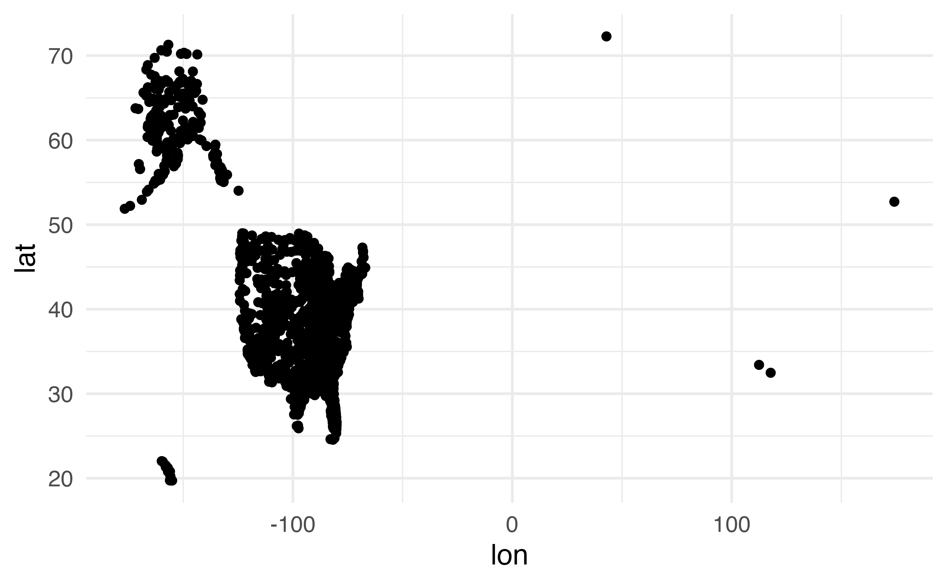
Let’s ignore the airports outside of the US.
airports |>
  filter(lon < 0) |>
  ggplot(aes(x = lon, y = lat)) +
  geom_point()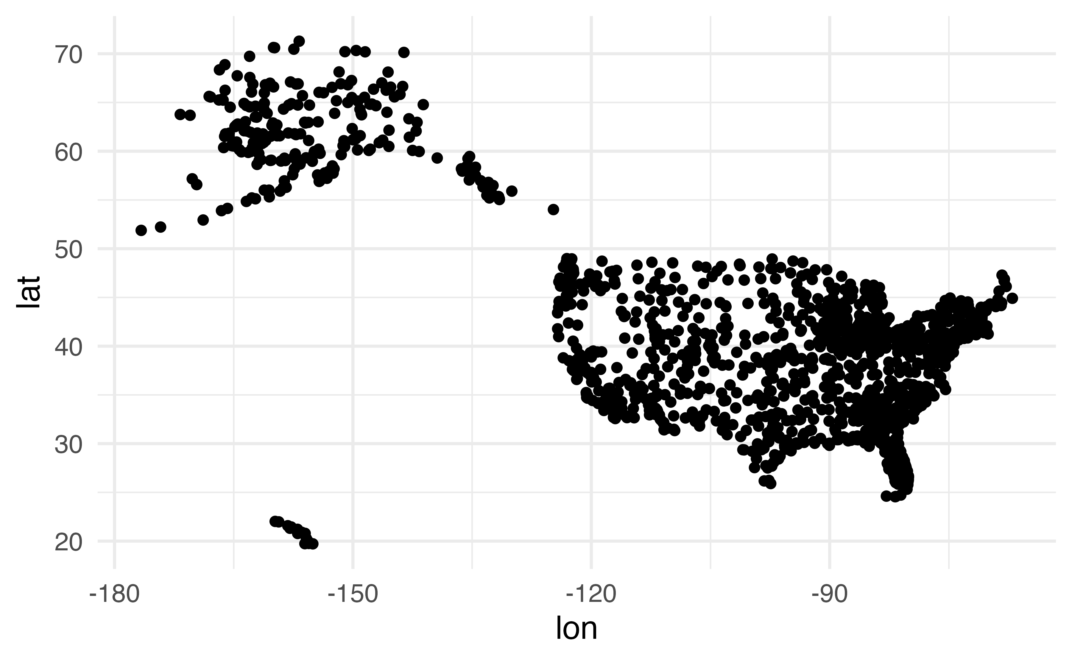
What does the ggplot() code translate to in SQL? Of course there is an error! SQL doesn’t have any plotting mechanism, so there couldn’t be any translation into SQL. Which reminds us that different programming languages have different advantages and disadvantages. The more we know about them, the better adept we will be at using the right language at the right time.
gg_query <- airports |>
  filter(lon < 0) |>
  ggplot(aes(x = lon, y = lat)) +
  geom_point()

show_query(gg_query)
Error in UseMethod("show_query"): no applicable method for 'show_query' applied to an object of class "c('gg', 'ggplot')"It is always a good idea to terminate the SQL connection when you are done with it.
dbDisconnect(con_air, shutdown = TRUE)What is the main purpose of a KEY? Can a KEY ever be NULL? (Hint: does it depend on what type of KEY it is?)
What is the main purpose of an INDEX? Can an INDEX ever be NULL?
How should we approach indexing? That is, what variables are good candidates for choosing to be the index?
Why is it harder to calculate the median than the mean?
Why are there three functions in R (ifelse(), case_when(), and cut()) to do the job of a single function in SQL (CASE WHEN)?
Why won’t dbplyr provide the syntax for the SQL translation of ggplot()?
What types of tasks is R best suited for? What types of tasks is SQL best suited for? Does it matter which one you use if they can both accomplish the same goal?
When setting up a database in SQL why is it important to consider potential users of the database and their potential questions / queries? That is, how is the set-up of the database related to the use of the database?