3 Maximum Likelihood Estimation
Maximum likelihood estimation is a method for choosing estimators of parameters that avoids using prior distributions or loss functions. MLE chooses \(\hat{\theta}\) as the estimate of \(\theta\) that maximizes the likelihood function (easily the most widely used estimation method in statistics).
Let’s say \(X \sim U[0, \theta].\) We collect \(X=47.\) Would you ever pick \(\theta=10?\) No! \(10 \notin \Omega!\)
Let’s say that \(X \sim\) Bin(\(\theta,\)n=4). If we have 4 independent trials, and X=1, would you chose \(\theta=0.99?\) But \(0.99 \in \Omega???\) You would choose \(\theta = 0.25.\) Why? Because you maximized the likelihood.
\[\begin{eqnarray*} P(X=1 | \theta = 0.25) &=& 0.422\\ P(X=1 | \theta = 0.5) &=& 0.25\\ P(X=1 | \theta = 0.05) &=& 0.171\\ P(X=1 | \theta = 0.15) &=& 0.368\\ \end{eqnarray*}\] You maximized the probability of seeing your data!
Example 3.1 Let’s say that houses on a block have their electricity connected in such a way that it only works for house #47 if all the neighbor’s electricity works (in sequence). Sometimes a house’s electricity will fail (w/prob p). To how many houses can we expect to provide electricity? What is our best guess of p?
Data: let’s say we have \(n\) neighborhoods with information on which house lost electricity. [What is the distribution of \(X?\) \(X \sim geometric(p),\) which means \(E[X] = 1/p.]\)
\[\begin{eqnarray*} f(x_i | p) &=& p (1-p)^{x_i -1}\\ f(\underline{x} | p) &=& \prod_{i=1}^n p (1-p)^{x_i -1}\\ &=& p^n (1-p)^{\sum x_i -n}\\ && \mbox{we want to maximize wrt } p \end{eqnarray*}\]
Often, the log-likelihood is easier to maximize than the likelihood. We define the log likelihood as \[\begin{eqnarray*} L(\theta) = \ln f(\underline{X} | \theta). \end{eqnarray*}\]
For example, \[\begin{eqnarray*} L(p) &=& \ln f(\underline{x} | p) = n \ln(p) + (\sum x_i -n) \ln(1-p)\\ \frac{\partial L(p)}{\partial p} &=& \frac{n}{p} + \frac{(\sum x_i -n)(-1)}{(1-p)} = 0\\ \hat{p} &=& \frac{1}{\overline{X}} \end{eqnarray*}\]
If \(\overline{x} = 10\), \(\hat{p} = 1/10\) (1 failure at 10 homes). E[X] = 1/p. (If we let \(\theta = E[X] -1\), then a good estimate of the expected (average) number of homes to which we can provide electricity is \(1/\hat{p} -1 = 10 - 1\). It turns out that the MLE has the invariance property which says that a function of the MLE is the MLE of that function of the parameter.)
Note that we’ve found a maximum: \[\begin{eqnarray*} \frac{\partial^2 L(p)}{\partial p^2} &=& \frac{2np -n -p^2\sum x_i}{p^2 (1-p)^2}\\ &\leq& \frac{2p n - n -p^2n}{p^2 (1-p)^2}\\ (\mbox{because } n &\leq& \sum x_i)\\ &=& \frac{n ( -2p + 1 +p^2}{p^2 (1-p)^2}\\ &=& \frac{-n}{p^2} < 0\\ \end{eqnarray*}\]
Definition 3.1 Maximum Likelihood Estimator (Def 7.5.2).
For each possible observed vector \(\underline{x}\), let \(\delta(\underline{x}) \in \Omega\) denote a value of \(\theta \in \Omega\) for which the likelihood function, \(f(\underline{x}|\theta)\) is a maximum, and let \(\hat{\theta} = \delta(\underline{X})\) be the estimator of \(\theta\) defined in this way. The estimator for \(\hat{\theta}\) is called a maximum likelihood estimator of \(\theta.\) After \(\underline{X} = \underline{x}\) is observed, the value \(\delta(\underline{x})\) is called a maximum likelihood estimate of \(\theta.\)
Sampling from a Normal Distribution
\[\begin{eqnarray*} X_1, X_2, \ldots X_n &\stackrel{iid}{\sim}& N(\mu, \sigma^2) \ \ \ \mu \ \& \ \sigma^2 \mbox{ are fixed but unknown}\\ f(x_i | \mu, \sigma^2) &=& \frac{1}{\sqrt{2 \pi \sigma^2}} \exp [ \frac{-1}{2\sigma^2}(x_i - \mu)^2 ]\\ f(\underline{x} | \mu, \sigma^2) &=& \frac{1}{(2 \pi \sigma^2)^{n/2}} \exp [ \frac{-1}{2\sigma^2}\sum_{i=1}^n(x_i - \mu)^2 ]\\ L(\mu, \sigma^2) &=& \frac{-n}{2}\ln(2\pi\sigma^2) - \frac{1}{2 \sigma^2} \sum(x_i - \mu)^2\\ \end{eqnarray*}\]
We want to maximize \(f(\underline{x}|\mu, \sigma^2)\) with respect to \(\mu;\) equivalently, we can minimize \(\sum (x_i - \mu)^2.\)
\[\begin{eqnarray*} \mbox{Let } Q(\mu) &=& \sum(x_i - \mu)^2\\ \frac{\partial Q(\mu)}{\partial \mu} &=& -2 \sum(x_i - \mu) = 0\\ -2 \sum x_i &=& -2 n \mu\\ \hat{\mu} &=& \overline{x} \end{eqnarray*}\]
Because the MLE for \(\mu\) doesn’t depend on \(\sigma^2\), we know that the joint MLE, \(\hat{\theta} = (\mu, \sigma^2)\), will be \(\hat{\theta}\) such that \(\hat{\sigma}^2\) maximizes (where \(\theta' = (\overline{x}, \sigma^2) ):\) \[\begin{eqnarray*} L(\theta') &=& \frac{-n}{2} \ln (2 \pi) - \frac{n}{2} \ln(\sigma^2) - \frac{1}{2\sigma^2} \sum(x_i - \overline{x})^2\\ \frac{\partial L(\theta')}{\partial \sigma^2} &=& \frac{-n}{2 \sigma^2} - \frac{1(-1)}{2 (\sigma^2)^2} \sum(x_i - \overline{x}) = 0\\ \sum (x_i - \overline{x})^2 &=& \frac{n(\sigma^2)^2}{\sigma^2}\\ \hat{\sigma^2} &=& \frac{\sum(x_i - \overline{x})^2}{n}\\ \hat{\theta} &=& (\overline{x}, \frac{\sum(x_i - \overline{x})^2}{n}) \end{eqnarray*}\]
Example 3.2 Non-existence of the MLE
Suppose \(X_1, X_2, \ldots X_n \stackrel{iid}{\sim} f(x | \theta)\) where: \[\begin{eqnarray*} f(x | \theta) = \left\{ \begin{array}{ll} e^{\theta - x} & x > \theta\\ 0 & x \leq \theta \\ \end{array} \right. \end{eqnarray*}\]
\(\theta\) is unknown, but \(-\infty < \theta < \infty\). Does the MLE exist? \[\begin{eqnarray*} f(\underline{x}|\theta) &=& e^{n \theta - \sum x_i} \ \ \ \ \ \forall x_i > \theta\\ L(\theta) &=& n \theta - \sum x_i \ \ \ \ \ \forall x_i > \theta\\ \frac{\partial L(\theta)}{\partial \theta} &=& n = 0 ?!?!?!\\ \end{eqnarray*}\]
We want to find the largest \(\theta\) such that \(\theta < x_i \ \ \forall x_i\). Is \(\hat{\theta} = \min x_i\)? No, because \(\theta < \min x_i!\) If, instead, \[\begin{eqnarray*} f (x | \theta) = \left\{ \begin{array}{ll} e^{\theta - x} & x \geq \theta\\ 0 & x < \theta \\ \end{array} \right. \end{eqnarray*}\]
MLE of \(\theta\) is \(\hat{\theta} = \min x_i\).
3.1 Qualities of the MLE
3.1.1 Invariance of the MLE
Theorem 3.1 (DeGroot and Schervish (2011) Theorem 6.6.1) Let \(\hat{\theta}\) be the MLE of \(\theta\), and let \(g(\theta)\) be a function of \(\theta\). Then an MLE of \(g(\theta)\) is \(g(\hat{\theta})\). (Proof: see page 427 in DeGroot & Schervish)
Proof. Let \(\hat{\theta}\) be the MLE of \(\theta\). Then we know that \[L(\hat{\theta}) = \max_{\theta \in \Omega} L(\theta).\]
We let \(g\) be a one-to-one function such that \(\psi = g(\theta) \in \Gamma\) (the image of \(\Omega\) under g). Then we can denote the inverse function of \(g\) as \[\theta = h(\psi).\]
We know that the MLE of \(\psi\) is \(\hat{\psi}\) where \[L(h(\hat{\psi})) = \max_{\psi \in \Gamma} L(h(\psi)).\]
But we know that \(L(\theta)\) is maximized at \(\hat{\theta}\). So \(L(h(\psi))\) must also be maximized at \(h(\psi) = \hat{\theta}\). \[\therefore h(\hat{\psi}) = \hat{\theta} \ \ \ \mbox{ or } \ \ \ \hat{\psi} = g(\hat{\theta}).\]
If \(g\) is not one-to-one, however, we need to redefine what we mean by likelihood. If \(g(\theta)\) is not one-to-one there may be many values of \(\psi\) that satisfy \[g(\theta) = \psi.\] (For example, the square function. n.b. \(g\) still has to be a function, so it can’t map to multiple values.)
In that case, the correspondence between the maximum over \(\psi\) and the maximum over \(\theta\) breaks down. E.g., if \(\hat{\theta}\) is the MLE for \(\theta\), there may be another value of \(\theta\), say \(\theta_0\) for which \(g(\hat{\theta}) = g(\theta_0).\)
We define the induced log likelihood function: \[L^*(t) = \max_{\theta \in G_t} \ln f(\underline{x} | \theta).\]
Let \(G\) be the image of \(\Omega\) under g, then \[G_t = \{ \theta: g(\theta) = t\} \ \ \forall t \in G.\]
We define the MLE of \(g(\theta)\) to be \(\hat{t}\) where \[L^*(\hat{t}) = \max_{t \in G} L^* (t).\]
The proof follows (page 427). [Note that above there are two maximizations. That is, the first maximization created the log likelihood function. The second maximization found the maximum of the function over the parameter space.]
Example 3.3 Functions of MLEs are MLEs also!
- standard deviation of a normal: \[\begin{eqnarray*} \sigma &=& \sqrt{\sigma^2}\\ \hat{\sigma} &=& \mbox{MLE}(\sigma) = \sqrt{\frac{\sum (x_i - \overline{x})^2}{n}} \end{eqnarray*}\]
- mean of a uniform: \[\begin{eqnarray*} X &\sim& U [\theta_1, \theta_2]\\ \mu &=& \frac{\theta_1 + \theta_2}{2}\\ \hat{\mu} &=& \mbox{MLE}(\mu) = \frac{\max(x_i) + \min(x_i)}{2} \end{eqnarray*}\]
3.1.2 Consistency of the MLE
Under certain regularity conditions, the MLE of \(\theta\) is consistent for \(\theta\). That is, \[\begin{eqnarray*} \hat{\theta} \stackrel{P}{\rightarrow} \theta\\ \stackrel{\lim}{ n \rightarrow \infty} P [ | \hat{\theta} - \theta | > \epsilon ] = 0 \end{eqnarray*}\]
where \(\hat{\theta}\) is a function of \(X\).
3.1.3 Bias of the MLE (section 7.7)
Previously, we discussed briefly the concept of bias:
Definition 3.2 Unbiased (page 428 of DeGroot & Schervish): Let \(\delta(X_1, X_2, \ldots, X_n)\) be an estimator of \(g(\theta)\). We say \(\delta(X_1, X_2, \ldots, X_n)\) is unbiased if: \[\begin{eqnarray*} E[ \delta(X_1, X_2, \ldots, X_n)] = g(\theta) \end{eqnarray*}\]
Note: bias \((\delta(\underline{X}) ) = E[ \delta(\underline{X})] - g(\theta)\).
Example 3.4 Let \(X_1, X_2, \ldots, X_n \sim N(\mu, \sigma^2)\). Recall, \(\hat{\sigma^2} = \frac{\sum(X_i - \overline{X})^2}{n}\) is the MLE. \[\begin{eqnarray*} E[\hat{\sigma^2}] &=& E \bigg[ \frac{\sum(X_i - \overline{X})^2}{n}\bigg]\\ &=& \frac{1}{n} E\bigg[ \sum (X_i - \mu + \mu - \overline{X})^2 \bigg]\\ &=& \frac{1}{n} E\bigg[ \sum (X_i - \mu)^2 + 2 \sum (X_i - \mu)(\mu - \overline{X}) + n(\mu - \overline{X})^2 \bigg]\\ &=& \frac{1}{n}\bigg\{ E\bigg[ \sum (X_i - \mu)^2 - n [(\overline{X} - \mu)^2 ] \bigg] \bigg\}\\ &=& \frac{1}{n} \bigg\{ \sum E (X_i - \mu)^2 - n E [(\overline{X} - \mu)^2 ] \bigg\}\\ &=& \frac{1}{n}\{ n \sigma^2 - n \frac{\sigma^2}{n} \}\\ &=& \frac{n-1}{n} \sigma^2 \Rightarrow \mbox{Biased!} \end{eqnarray*}\]
But consistent? Yes.
\[\begin{eqnarray*} \frac{\sum(X_i - \overline{X})^2}{n} &=& \frac{1}{n}\bigg[ \sum (X_i - \mu)^2 - n [(\overline{X} - \mu)^2] \bigg] \\ &=& \frac{\sum(X_i - \mu)^2}{n} - \frac{1}{n} \frac{\sum n (\overline{X} - \mu)^2}{n}\\ &=& \stackrel{P}{\rightarrow} \sigma^2 \ \ \ \ \ \ \ \ \ \ \ \rightarrow 0 \ \ \ \stackrel{P}{\rightarrow} \sigma^2\\ &\stackrel{P}{\rightarrow}& \sigma^2\\ \end{eqnarray*}\]
3.1.4 Benefits and Limitations of Maximum Likelihood Estimation
Benefits
- functions of MLEs are MLEs (invariance of the MLE)
- under certain regularity conditions, MLEs are asymptotically distributed normally.
Limitations
- MLE does not always exist
- MLE is not always unique
- MLE is the value of the parameter \(\theta\) that maximizes the distribution of \(X|\theta\) (most likely to have produced the observed data). The MLE is not the most likely parameter given the data: \(E[ \theta | X]\) (that’s the Bayesian estimator!).
3.2 Method of Moments
Method of Moments (MOM) is another parameter estimation technique. To find the MOM estimate, set the expected moment equal to the sample moment and solve for the parameter value of interest.
\[\begin{eqnarray*} E[X^k] &=& k^{th} \mbox{ expected moment}\\ \frac{1}{n} X_i^k &=& k^{th} \mbox{ sample moment}\\ \end{eqnarray*}\]
Example 3.5 Find the MOM for both parameters using a random sample, \(X_1, X_2, \ldots, X_n \sim N(\mu, \sigma^2)\). \[\begin{eqnarray*} \tilde{\mu} &=& \overline{X}\\ \tilde{\sigma^2} &=& \frac{\sum X_i^2}{n} - \overline{X}^2\\ &=& \frac{1}{n} \sum(X_i - \overline{X})^2 \mbox{ MLE!!} \end{eqnarray*}\]
Example 3.6 Find the MOM for both parameters using a random sample, \(X_1, X_2, \ldots, X_n \sim Gamma(\alpha,\beta)\). \[\begin{eqnarray*} \alpha / \beta &=& \overline{X}\\ \alpha / \beta^2 &=& \sum X_i^2 /n - \overline{X}^2\\ \alpha &=& \overline{X} \beta\\ \frac{\overline{X} \beta}{\beta^2} &=& \sum X_i^2 /n - \overline{X}^2\\ \tilde{\beta} &=& \frac{\overline{X}}{(\sum X_i^2 / n - \overline{X}^2)}\\ &=& \overline{X} / \hat{\sigma^2}\\ \tilde{\alpha} &=& \overline{X}^2 / \hat{\sigma^2} \end{eqnarray*}\]
3.2.1 Benefits and Limitations of Method of Moments Estimation
Benefits
- Often easier to compute than MLEs (e.g., MLE for \(\alpha\) in the Gamma distribution is intractable).
- Estimates by MOM can be used as first approximations of the likelihood.
- Can easily estimate multiple parameter families.
Limitations
- Can sometimes (usually in cases of small sample sizes) produce estimates outside the parameter space.
- Doesn’t work if the moments don’t exist (e.g., Cauchy distribution)
- MLEs are typically closer to the quantity being estimated.
Example 3.7 Tank Estimators
How can a random sample of integers between 1 and N (with N unknown to the researcher) be used to estimate N?
- The tanks are numbered from 1 to N. Working with your group, randomly select five tanks, without replacement, from the bowl. The tanks are numbered:
- Think about how you would use your data to estimate N. (Come up with at least 3 estimators.) Come to a consensus within the group as to how this should be done.
- Our estimates of N are:
- Our rules or formulas for the estimators of N based on a sample of n (in your case 5) integers are:
- Assuming the random variables are distributed according to a discrete uniform: \[\begin{eqnarray*} X_i \sim P(X=x | N) = \frac{1}{N} \ \ \ \ \ x = 1,2,\ldots, N \ \ \ \ i=1,2,\ldots, n \end{eqnarray*}\]
- What is the method of moments estimator of N?
- What is the maximum likelihood estimator of N?
Mean Squared Error
Most of our estimators are made up of four basic functions of the data: the mean, the median, the min, and the max. Fortunately, we know something about the moments of these functions:
| g(\(\underline{X}\)) | E[ g(\(\underline{X}\)) ] | Var( g(\(\underline{X}\)) ) |
|---|---|---|
| \(\overline{X}\) | \(\frac{N+1}{2}\) | \(\frac{(N+1)(N-1)}{12 n}\) |
| median(\(\underline{X}\)) = M | \(\frac{N+1}{2}\) | \(\frac{(N-1)^2}{4 n}\) |
| min(\(\underline{X}\)) | \(\frac{(N-1)}{n} + 1\) | \(\bigg(\frac{N-1}{n}\bigg)^2\) |
| max(\(\underline{X}\)) | \(N - \frac{(N-1)}{n}\) | \(\bigg(\frac{N-1}{n}\bigg)^2\) |
Using this information, we can calculate the MSE for 4 of the estimators that we have derived. (Remember that MSE = Variance + Bias\(^2\).)
\[\begin{eqnarray} \mbox{MSE } ( 2 \cdot \overline{X} - 1) &=& \frac{4 (N+1) (N-1)}{12n} + \Bigg(2 \bigg(\frac{N+1}{2}\bigg) - 1 - N\Bigg)^2 \nonumber \\ &=& \frac{4 (N+1) (N-1)}{12n} \\ \nonumber \\ \mbox{MSE } ( 2 \cdot M - 1) &=& \frac{4 (N-1)^2}{4n} + \Bigg(2 \bigg(\frac{N+1}{2}\bigg) - 1 - N\Bigg)^2 \nonumber \\ &=& \frac{4 (N-1)^2}{4n} \\ \nonumber \\ \mbox{MSE } ( \max(\underline{X})) &=& \bigg(\frac{N-1}{n}\bigg)^2 + \Bigg(N - \frac{(N-1)}{n} - N\Bigg)^2 \nonumber\\ &=& \bigg(\frac{N-1}{n}\bigg)^2 + \bigg(\frac{N-1}{n} \bigg)^2 = 2*\bigg(\frac{N-1}{n} \bigg)^2 \\ \nonumber \\ \mbox{MSE } \Bigg( \bigg( \frac{n+1}{n} \bigg) \max(\underline{X})\Bigg) &=& \bigg(\frac{n+1}{n}\bigg)^2 \bigg(\frac{N-1}{n}\bigg)^2 + \Bigg(\bigg(\frac{n+1}{n}\bigg) \bigg(N - \frac{N-1}{n} \bigg) - N \Bigg)^2 \end{eqnarray}\]
3.3 Reflection Questions
- What function is being maximized when an MLE is found? Derivative with respect to what? That is, explain the intuition behind why the MLE is a good estimator for \(\theta.\)
- How is the MOM estimator found? Explain why the MOM is a good estimator for \(\theta.\)
- What are the asymptotic properties of the MLE that make it nice to work with?
- What are the benefits and limitations of the MLE?
- What are the benefits and limitations of MOM?
3.4 Ethics Considerations
- Does the derivative always work to find the MLE? If not, what other ways can we find a maximum?
- Is the MLE always the best estimator for \(\theta\)?
- Is the MOM always the best estimator for \(\theta\)?
- What makes a good estimator?
- You are consulting, you are given a dataset, you are asked to find \(\theta\), is there a single right answer? How do you know what to give your boss?
- What do you do if you have a dataset but you don’t know the likelihood?
3.5 R code: MLE Example
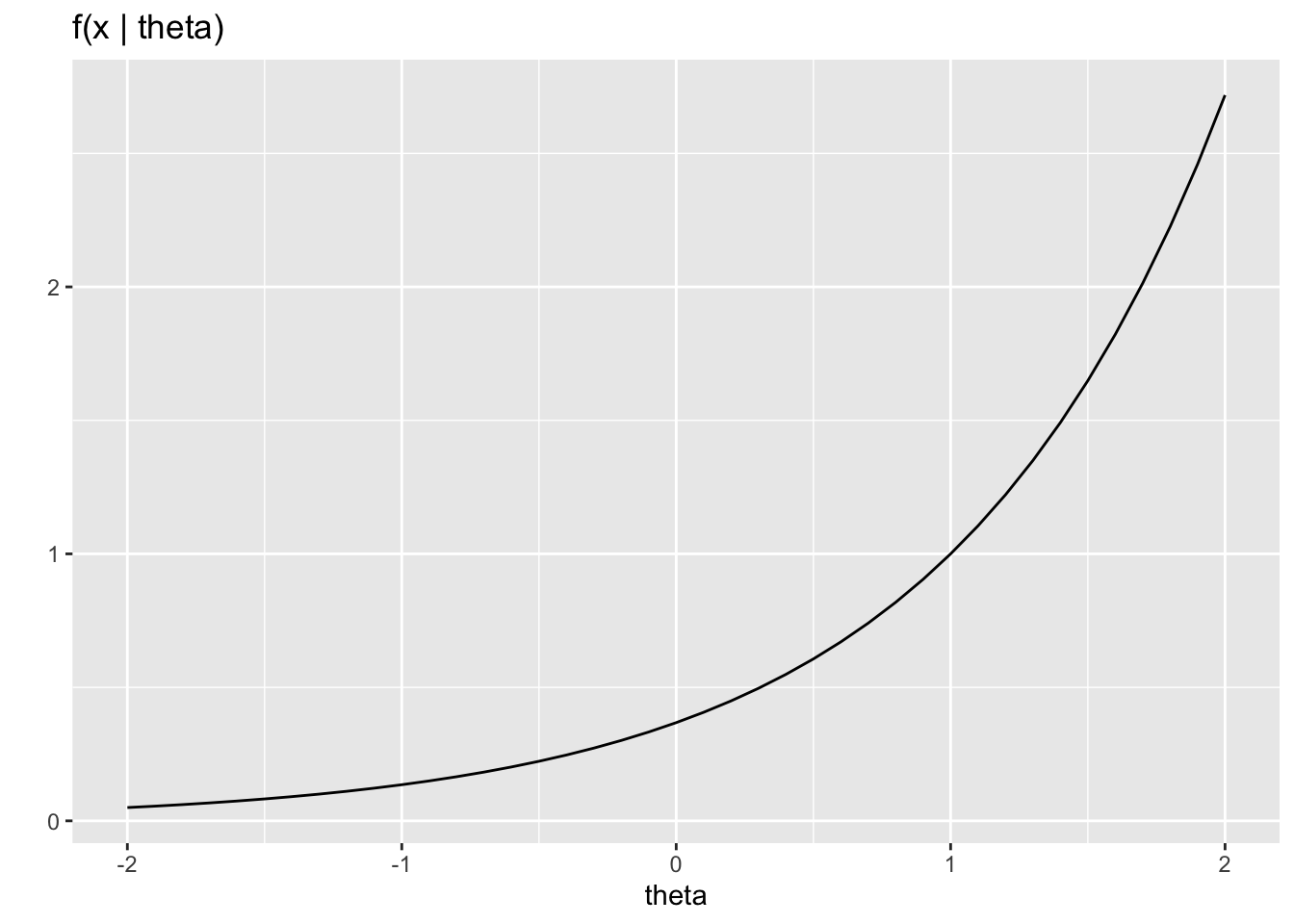
Example 7.6.5 in the text looks at the MLE for the center of of a Cauchy distribution. The Cauchy distribution is interesting because the tails decay at a rate of \(1/x^2\), so that when you try to take the expected value, you end up integrating something that looks like \(1/x\) over the real line. Hence, the expected value does not exist. Thus, method of moments estimators are of no use. The MLE is still useful, though not easy to find. As stated in the text, the likelihood is proportional to \[\prod_{i=1}^n [1 + (x_i - \theta)^2]^{-1}\]
- Compute the first and second derivative of the log likelihood.
- Consider trying to find the root of a function \(h(x)\). Suppose your current guess is some value \(x_0\). We might approximate the function by the tangent line (first order Taylor approximation) at \(x_0\) and take our next guess as the root of that line. Use the Taylor expansion to find the next guess of \(x_1\) as
\[x_1 = x_0 - \frac{h(x_0)}{h'(x_0)}\]
Continually updating the guess via this method is known as Newton’s Method or the Newton-Raphson Method.
- Generate 50 observations from a Cauchy distribution centered at \(\theta = 10\). Based on these 50 observations, use parts (a) and (b) to estimate \(\theta\). Remember, we’re trying to maximize the likelihood, so the function that we are trying to find the root of is derivative of the log-likelihood. The R code might look something like this:
The Cauchy distribution is very sensitive to the initial value used in Newton’s method, so if your theta_guess is not very close to 10, probably the MLE estimate will be infinite.
library(tidyverse)

# Use Newton's method to find the MLE for a Cauchy distribution
cauchy_mle <- function(guess, data){
    l1 <- ((compute 1st derivative of log-likelihood evaluated at "guess")) # 1st deriv
    l2 <- ((compute 2nd derivative of log-likelihood evaluated at "guess")) # 2nd deriv
    guess <- guess - l1/l2
    guess
}

# set up the initial conditions (including the dataset to use)
set.seed(54321)  # to get the same answer each time the .Rmd is knit

n_obs <- 50
observations <- rcauchy(n_obs, location = 10)  # 50 random Cauchy, centered at 10
theta_guess <- ((pick a starting value, you might try different ones)) # just a number
Running cauchy_mle recursively
theta_guess <- 10
guess_vec <- numeric()
reps <- 10  # play around with how many times you loop through.
# you probably don't need very many times through to see what happens.
# what happens might seem unsettling!

for(i in 1:reps){
  theta_guess <- cauchy_mle(___, ___)  # what changes for each rep?
  guess_vec[i] <- theta_guess
}
guess_vec

data.frame(guess_vec) %>%  # ggplot needs a data frame instead of a vector
  ggplot(aes(y = guess_vec, x = 1:reps)) +
  geom_line()  # line plot connecting the guesses for each rep
Reflection
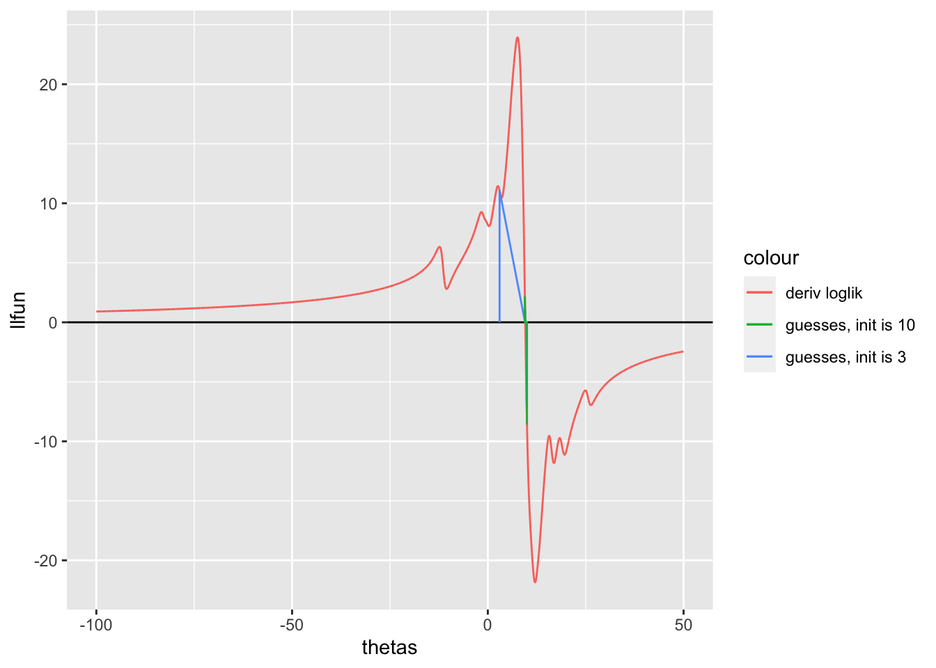
Just for kicks, I’ve plotted the derivative of the log-likelihood (red, trying to find the zero of the derivative of the log-likelihood) as well as two different guess trajectories (green from start of 10 and blue from a start of 3). The green line (hard to see, look right at theta = 10) indicates that we get to the maximum if we are very close to 10 as a start. The blue line indicates what happens if the initial value is far from 10 (the MLE is estimated to be infinite).
I’ve left in the R code, but don’t worry about understanding the specific lines of code. Instead focus on understanding the image itself. It should tell you that the function does have a maximum (i.e., the derivative goes through zero!), but that the x-value for which the derivative equals zero is difficult to find. Using the Newton-Raphson method requires that the initial guess is quite close to the truth, otherwise, the estimate will go to positive or negative infinity.
set.seed(470)
n_obs <- 50
observations <- rcauchy(n_obs, location = 10)  # 50 random Cauchy, centered at 10


# print the derivative of the log likelihood function
# this is what you're trying to find the zero of
thetas <-  seq(-100,50,by = .01)
llfun <-  c()
for (k in 1:length(thetas))
{
llfun[k] <- 2*sum((observations-thetas[k])/(1+(observations-thetas[k])^2))
}


# draw on top two instances of Newton's method:
# starting at theta_guess = 10  (RED)
theta_guess <- 10
theta_10 <- 10
l1_vals_10 <- c(0)
for (i in 1:5)
    {
    l1 <- 2*sum((observations-theta_guess)/(1+(observations-theta_guess)^2))
    l2 <- 2*sum((-1+(observations-theta_guess)^2)/(1+(observations-theta_guess)^2)^2)
    theta_next <- theta_guess - l1/l2
    theta_guess <- theta_next
    theta_10[i + 1] <- theta_guess
    l1_vals_10 <- c(l1_vals_10, l1, 0)
    }


# then starting at theta_guess = 3 (PURPLE)
theta_guess <- 3
theta_3 <- 3
l1_vals_3 <- c(0)
for (i in 1:5)
  {
    l1 <- 2*sum((observations-theta_guess)/(1+(observations-theta_guess)^2))
    l2 <- 2*sum((-1+(observations-theta_guess)^2)/(1+(observations-theta_guess)^2)^2)
    theta_next <- theta_guess - l1/l2
    theta_guess <- theta_next
    theta_3[i + 1] <- theta_guess
    l1_vals_3 <- c(l1_vals_3, l1, 0)
}


guesses_10 <- data.frame(thetas = rep(theta_10, each = 2),
                        guess = c(l1_vals_10,0))
guesses_3 <- data.frame(thetas = rep(theta_3, each = 2),
                        guess = c(l1_vals_3,0))
cauchy_data <- data.frame(thetas, llfun)


cauchy_data %>%
  ggplot() +
  geom_hline(yintercept = 0) +
  geom_line(aes(x = thetas, y = llfun, color = "deriv loglik")) +
  geom_line(data = guesses_3, aes(x = thetas, y = guess, color = "guesses, init is 3")) +
  geom_line(data = guesses_10, aes(x = thetas, y = guess, color = "guesses, init is 10")) +
  xlim(c(-100, 50))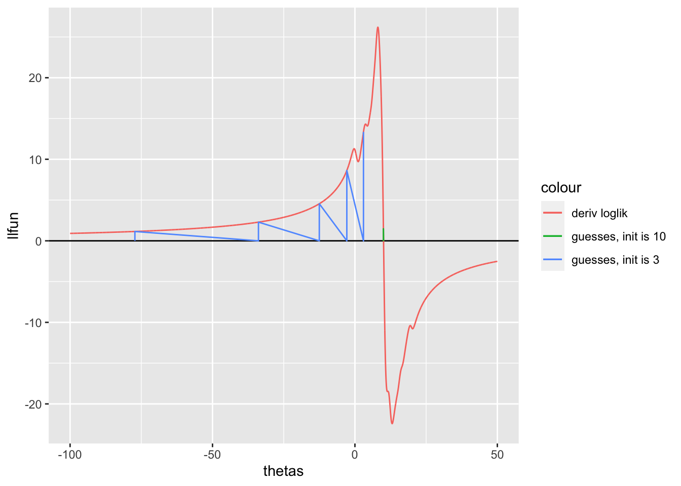
Odd things happen sometimes
I’ve run this code many many many times over the years. And every time, if the initial guess is not super close to 10, the estimate doesn’t converge. But just once, I set the seed in a particular way, and the start value of 3 actually converged to the answer! Randomness in the wild.
set.seed(4747)
n_obs <- 50
observations <- rcauchy(n_obs, location = 10)  # 50 random Cauchy, centered at 10


# print the derivative of the log likelihood function
# this is what you're trying to find the zero of
thetas <-  seq(-100,50,by = .01)
llfun <-  c()
for (k in 1:length(thetas))
{
llfun[k] <- 2*sum((observations-thetas[k])/(1+(observations-thetas[k])^2))
}


# draw on top two instances of Newton's method:
# starting at theta_guess = 10  (RED)
theta_guess <- 10
theta_10 <- 10
l1_vals_10 <- c(0)
for (i in 1:5)
    {
    l1 <- 2*sum((observations-theta_guess)/(1+(observations-theta_guess)^2))
    l2 <- 2*sum((-1+(observations-theta_guess)^2)/(1+(observations-theta_guess)^2)^2)
    theta_next <- theta_guess - l1/l2
    theta_guess <- theta_next
    theta_10[i + 1] <- theta_guess
    l1_vals_10 <- c(l1_vals_10, l1, 0)
    }


# then starting at theta_guess = 3 (PURPLE)
theta_guess <- 3
theta_3 <- 3
l1_vals_3 <- c(0)
for (i in 1:5)
  {
    l1 <- 2*sum((observations-theta_guess)/(1+(observations-theta_guess)^2))
    l2 <- 2*sum((-1+(observations-theta_guess)^2)/(1+(observations-theta_guess)^2)^2)
    theta_next <- theta_guess - l1/l2
    theta_guess <- theta_next
    theta_3[i + 1] <- theta_guess
    l1_vals_3 <- c(l1_vals_3, l1, 0)
}


guesses_10 <- data.frame(thetas = rep(theta_10, each = 2),
                        guess = c(l1_vals_10,0))
guesses_3 <- data.frame(thetas = rep(theta_3, each = 2),
                        guess = c(l1_vals_3,0))
cauchy_data <- data.frame(thetas, llfun)


cauchy_data %>%
  ggplot() +
  geom_hline(yintercept = 0) +
  geom_line(aes(x = thetas, y = llfun, color = "deriv loglik")) +
  geom_line(data = guesses_3, aes(x = thetas, y = guess, color = "guesses, init is 3")) +
  geom_line(data = guesses_10, aes(x = thetas, y = guess, color = "guesses, init is 10")) +
  xlim(c(-100, 50))